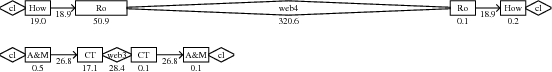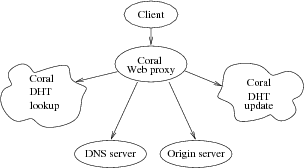
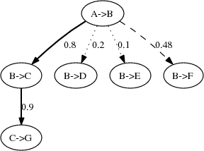
Figure 1: Example causal path through Coral.
Wide-area distributed systems are difficult to build and deploy because traditional debugging tools do not scale across multiple processes, machines, and administrative domains. Compared to local-area distributed systems, wide-area distributed systems introduce new sources of delays and failures, including network latency, limited bandwidth, node unreliability, and parallel programming. Furthermore, the sheer size of a wide-area system can make it daunting to find and debug underperforming nodes or to examine event traces. Often, programmers have trouble understanding the communications structure of a complex distributed system and have trouble isolating the specific sources of delays.
In this paper, we present the Wide-Area Project 5 (WAP5) system, a set of tools for capturing and analyzing traces of wide-area distributed applications. The WAP5 tools aid the development, optimization, and maintenance of wide-area distributed applications by revealing the causal structure and timing of communication in these systems. They highlight bottlenecks in both processing and communication. By mapping an application's communication structure, they highlight when an application's data flow follows an unexpected path. By discovering the timing at each step, they isolate processing or communication hotspots.
We are focusing on applications running on PlanetLab [3], perhaps the best collection of widely distributed applications for which research access is feasible. In particular, we have applied our tools to the CoDeeN [19] and Coral [7] content-distribution networks (CDNs). WAP5 constructs causal structures, such as the one shown for Coral in Figure 1, which matches a path described by Figure 1 in a paper on Coral [7].
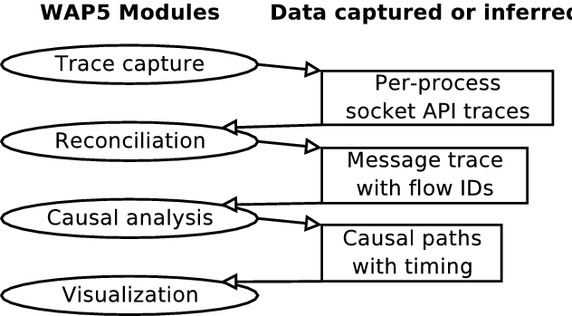
Our tool chain consists of four steps, depicted in Figure 2. First, our dynamically linked interposition library captures one trace of socket-API calls per application process on each participating machine. Second, we reconcile the socket-API traces to form a single trace with one record per message containing both a sent and a received timestamp. These timestamps reflect the clocks at the sender and receiver machines, respectively, and are used to quantify and compensate for clock skew and to measure network latency. Third, we run our causality analysis algorithm on the reconciled trace to find causal paths through the application, like the one in Figure 1. Finally, we render the causal paths as trees or timelines.
In the space of tools that analyze application behavior for performance debugging, our approach is among the least invasive and works on the largest scale of systems: wide-area distributed systems. Other causal-path analysis tools differ in their invasiveness or in the scale of systems they target. Our earlier work [1], known as Project 5, targets heterogeneous local-area distributed systems and is minimally invasive because it works using only network traces. Magpie [2] and Pinpoint [4] target (mostly) homogeneous local-area distributed systems and require specific platforms with the appropriate logging capabilities. In some cases, Pinpoint also requires the ability to change message formats. DPM [10] traces single-computer systems using an instrumented kernel. Pip [13] supports wide-area systems but requires manual annotations, an instrumented platform, or both. We discuss related work further in Section 8.
This paper makes the following contributions:
In the next section, we define the problem we are solving more explicitly. We then describe the three main tools in our approach, which perform trace capture, trace reconciliation, and causal path analysis over the trace. Finally, we present results from three systems.
In this section, we define the problem we are solving. We include a description of the target applications, discussion of some distributed hash table (DHT) issues, definitions of our terminology for communication between components, our model of causality, and several issues related to naming of components.
Our primary goal is to expose the causal structure of communication within a distributed application and to quantify both processing delays inside nodes and communication (network) delays. In this paper, we specifically focus on wide-area distributed systems (and other systems) where the network delays are non-negligible. We further focus on PlanetLab applications because we can get access to them easily. However, nothing in our approach requires the use of PlanetLab.
We aim to use as little application-specific knowledge as possible and not to change the application. We can handle applications whose source code is unavailable, whose application-level message formats are unknown, and, in general, without a priori information about the design of the application.
Our tools can handle distributed systems whose ``nodes'' span a range of granularities ranging from entire computers down to single threads, and whose communication paths include various network protocols and intra-host IPC. We aim to support systems that span multiple implementation frameworks; for example, a multi-tier application where one tier is J2EE, another is .Net, and a third is neither.
We currently assume the use of unicast communications and we assume that communication within an application takes the form of messages. It might be possible to extend this work to analyze multicast communications.
Several interesting distributed applications are based on DHTs. Therefore, we developed some techniques specifically for handling DHT-based applications.
DHTs perform lookups either iteratively, recursively, or
recursively with a shortcut response [5]. In an iterative lookup,
the node performing the query contacts several remote hosts
(normally ![]() for systems with
for systems with ![]() total hosts)
sequentially, and each provides a referral to the next. In a
recursive lookup, the node performing the query contacts one
host, which contacts a second on its behalf, and so on. A
recursive lookup may return back through each intermediary, or it
may return directly along a shortcut from the destination node
back to the client.
total hosts)
sequentially, and each provides a referral to the next. In a
recursive lookup, the node performing the query contacts one
host, which contacts a second on its behalf, and so on. A
recursive lookup may return back through each intermediary, or it
may return directly along a shortcut from the destination node
back to the client.
With an iterative DHT, all of the necessary messages for analysis of causal paths starting at a particular node can be captured at that node. With a recursive or recursive-shortcut DHT, causal path analysis requires packet sniffing or instrumentation at every DHT node. The algorithm presented in this paper handles all three kinds of DHT.
DHTs create an additional ``aggregation'' problem that we defer until Section 2.5.1.
Networked communication design typically follows a layered architecture, in which the protocol data units (PDUs) at one layer might be composed of multiple, partial, or overlapping PDUs at a lower layer. Sometimes the layer for meaningfully expressing an application's causal structure is higher than the layer at which we can obtain traces. For example, in order to send a 20 KB HTTP-level response message, a Web server might break it into write() system call invocations based on an 8 KB buffer. The network stack then breaks these further into 1460-byte TCP segments, which normally map directly onto IP packets, but which might be fragmented by an intervening router.
We have found it necessary to clearly distinguish between messages at different layers. In this paper, we use the term packet to refer to an IP or UDP datagram or a TCP segment. We use message to refer to data sent by a single write() system call or received by a single read(). We refer to a large application-layer transfer that spans multiple messages as a fat message. Fat messages require special handling: we combine adjacent messages in a flow into a single large message before beginning causal analysis. Conversely, several sufficiently small application-layer units may be packed into a single system call or network packet, in protocols that allow pipelining. In the systems analyzed here, such pipelining does not occur. In systems where pipelining is present, our tool chain would see fewer requests than were really sent but would still find causality.
We consider message A to have caused message B if message A is
received by node X, message B is sent by node X, and the logic in
node X is such that the transmission of B depends on receiving A.
In our current work, we assume that every message B is either
caused by one incoming message A or is spontaneously generated by
node X. This assumption includes the case where message A causes
the generation of several messages
![]() .
.
An application where one message depends on the arrival of many messages (e.g., a barrier) does not fit this model of causality. WAP5 would attribute the outgoing message to only one--probably the final--incoming message. Additionally, if structure or timing of a causal path pattern depends on application data inside a message, WAP5 will view each variation as a distinct path pattern and will not detect any correlation between the inferred path instances and the contents of messages.
We cannot currently handle causality that involves asynchronous timers as triggers; asynchronous events appear to be spontaneous rather than related to earlier events. This restriction has not been a problem for the applications we analyzed for this paper. We also cannot detect that a node is delayed because it is waiting for another node to release a lock.
Our trace-based approach to analyzing distributed systems exposes the need for multiple layers of naming and for various name translations. Clear definitions of the meanings of various names simplify the design and explanation of our algorithms and results. They also help us define how to convert between or to match various names.
Causal path analysis involves two categories of named objects, computational nodes and communication flow endpoints. Nodes might be named using hostnames, process IDs, or at finer grains. Endpoints might be named using IP addresses, perhaps in conjunction with TCP or UDP ports, or UNIX-domain socket pathnames. These multiple names lead to several inter-related challenges:
The selection of naming granularity interacts with the choice of tracing technology. Packet sniffing, the least invasive tracing approach, makes it difficult or impossible to identify processes rather than hosts. Use of an interposition library, such as the one we describe in Section 3, allows process-level tracing.
The distinction between node names and endpoint names allows the analysis of a single distributed application by using multiple traces obtained with several different techniques. For example, we could trace UNIX-domain socket messages using the interposition library and simultaneously trace network messages using a packet sniffer.
Table 1: Where different naming information is captured (C) or used (U).
| Socket API parameters | Other captured information | ||||||||
|---|---|---|---|---|---|---|---|---|---|
| both ends: (IP addr,port) | socket path | file descriptor | length | hostname | PID | peer PID | checksum | timestamp | |
| trace file header | C | C | C | ||||||
| new connection: TCP | C | C | C | ||||||
| new connection: UDP or raw IP | C | C | C | ||||||
| new connection: UNIX domain | C | C | C | C | |||||
| message: TCP or UNIX domain | C | C | C | ||||||
| message: UDP or raw IP | C | C | C | C | C | ||||
| reconciliation: matching send & rcv recs | U | U | U | U | U | U | |||
| causal analysis (message linking) | U | U | U | ||||||
| aggregating nodes | U | U | |||||||
Table 1 shows the various names (the columns) captured by our interposition library, and where they are used in our analysis. We include this table to illustrate the complexity of name resolution; it may be helpful to refer to it when reading Sections 4 and 5.
Causal path analysis aggregates similar path instances into path patterns, presenting to the user a count of the instances inferred along with average timing information. The simplest form of aggregation is combining path instances with identical structure, i.e., those that involve exactly the same nodes in exactly the same order. More advanced aggregation techniques look for isomorphic path instances that perform the same tasks via different nodes, perhaps for load balancing. Without aggregation, it is difficult to visualize how a system performs overall: where the application designer thinks of an abstract series of steps through an application, causal path analysis finds a combinatorial explosion of rare paths going through specific nodes. Aggregation is particularly important for DHTs, which are highly symmetric and use an intentionally wide variety of paths for reliability and load balancing. Aggregating paths is useful for finding performance bugs that are due to a design or coding error common to all hosts.
Figure 3: Example of aggregation across multiple names
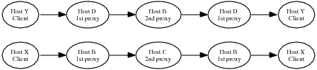
(a) unaggregated paths

(b) corresponding aggregated path
Once causal path analysis has identified a set of isomorphic paths, it is possible to aggregate the results based on the role of a node rather than its name. For example, Coral and CoDeeN have thousands of clients making requests; trees starting at one client would not normally be aggregated with trees starting at another. As another example, Figure 3(a) shows two causal paths with the same shape but different hostnames. In the top path, Host D fills the role of the first-hop proxy, and Host B fills the role of the second-hop proxy; in the other path, Host B is the first-hop proxy and and Host C is the second-hop proxy. What we might like to see instead is the aggregated path in Figure 3(b), which aggregates the clients, first-hop, and second-hop proxies. Of course, the unaggregated paths should still be available, in case a performance problem afflicts specific nodes rather than a specific task.
Currently, our code aggregates clients, but we have not yet implemented aggregation across servers. To aggregate clients, we designate each TCP or UDP port as fixed or ephemeral and each node as a client or a server. A port is fixed if it communicates with many other ports. For example, a node making a DNS request will allocate a source port dynamically (normally either sequentially or randomly), but the destination port will always be 53. Thus, causal path analysis discovers that 53 is a fixed port because it talks to hundreds or thousands of other ports. A node is considered a server if it uses fixed ports at least once, and a client otherwise. Our algorithm replaces all client node names with a single string ``CLIENT'' and replaces all ephemeral port numbers with an asterisk before building and aggregating trees. Thus, otherwise identical trees beginning at different clients with different ephemeral source-port numbers can be aggregated.
We now describe how we capture traces of inter-node
communication. We wrote an interposition library, LibSockCap, to
capture network and inter-process communication. LibSockCap
captures mostly the same information as strace -e network (i.e., a trace of all
networking system calls), plus additional needed information with
much lower overhead. The extra information is needed for
reconciliation and includes fingerprints of UDP message contents,
the PID of peers connecting through a Unix socket, the peer name
even when accept does not ask for it,
the local name bound when connect is
called, and the number assigned to a dynamic listening port not
specified with bind. Further,
LibSockCap imposes less than 2![]() of overhead per captured system call,
while strace imposes up to 60
of overhead per captured system call,
while strace imposes up to 60![]() of overhead per system call. Finally,
LibSockCap generates traces about an order of magnitude smaller
than strace.
of overhead per system call. Finally,
LibSockCap generates traces about an order of magnitude smaller
than strace.
LibSockCap traces dynamically linked applications on any platform that supports library interposition via LD_PRELOAD. LibSockCap interposes on the C library's system call wrappers to log all socket-API activity, for one or more processes, on all network ports and also on UNIX-domain sockets. For each call, LibSockCap records a timestamp and all parameters (as shown in Table 1), but not the message contents. In addition, LibSockCap monitors calls to fork so that it can maintain a separate log for each process. On datagram sockets, it also records a message checksum so that dropped, duplicated, and reordered packets can be detected.
There are several advantages to capturing network traffic through library interposition rather than through packet sniffing, either on each host or on each network segment.
Interposition does have disadvantages relative to sniffing.
The advantages are significant enough that even in environments where sniffing is feasible, we prefer to use LibSockCap.
To verify that LibSockCap imposes negligible overhead on the applications being traced, we ran Seda's HttpLoad [20] using Java 1.4.1_01 against Apache 1.3.1. Both the client and the server were dual 2.4 GHz Pentium 4 Xeon systems running Linux 2.4.25. LibSockCap had no measurable effect on throughput or on average, 90th-percentile, or maximum request latency for any level of offered load. However, the server CPU was not saturated during this benchmark, so LibSockCap might have more impact effect on a CPU-bound task.
We measured the absolute overhead of LibSockCap by comparing
the time to make read/write system calls with and without
interposition active, using the server described above.
LibSockCap adds about 0.02![]() of overhead to file reads and writes,
which generate no log entries; 1.03
of overhead to file reads and writes,
which generate no log entries; 1.03![]() to TCP reads;
1.02
to TCP reads;
1.02![]() to
TCP writes; and 0.75
to
TCP writes; and 0.75![]() to UDP writes. In our benchmark, Apache made
at most 3,019 system calls per second, equal to an overhead of
about 0.3% of one CPU's total cycles.
to UDP writes. In our benchmark, Apache made
at most 3,019 system calls per second, equal to an overhead of
about 0.3% of one CPU's total cycles.
To capture the traces used for our experiments, we sent LibSockCap sources to the authors of Coral and CoDeeN. Both reported back that they used their existing deployment mechanisms to install LibSockCap on all of their PlanetLab nodes. After the processes ran and collected traces for a few hours, they removed LibSockCap, retrieved the traces to a single node, and sent them to us.
While LibSockCap is more invasive than packet sniffing (in that it requires additional software on each node), packet sniffing is more logistically challenging in practice, as we discuss in Section 7.
The trace reconciliation algorithm converts a set of per-process traces of socket activity (both network and inter-process messages) to a single, more abstract, trace of inter-node messages. This algorithm includes translation from socket events to flow-endpoint names and node names. The output is a trace containing logical message tuples of the form (sender-timestamp, sender-endpoint, sender-node, receiver-timestamp, receiver-endpoint, receiver-node).
Name translation: In the
LibSockCap traces, each send or recv event
contains a timestamp, a size, and a file descriptor.
Reconciliation converts each file descriptor to a flow-endpoint
name. With UNIX domain and TCP sockets, we can easily find the
flow-endpoint name (i.e., UNIX path or ![]() IP address,
port
IP address,
port![]() pair) in prior connect, accept, or
bind API events in the trace. File descriptors for
datagram (UDP or raw IP) sockets, however, may or may not be
bound to set source and destination addresses. If not, the remote
address is available from the sendto or
recvfrom parameter and we use the host's public IP
address or the loopback address as the local address.
pair) in prior connect, accept, or
bind API events in the trace. File descriptors for
datagram (UDP or raw IP) sockets, however, may or may not be
bound to set source and destination addresses. If not, the remote
address is available from the sendto or
recvfrom parameter and we use the host's public IP
address or the loopback address as the local address.
Timestamps: We include the timestamps from both the sender and receiver traces in the final trace. With both timestamps, it is simple to obtain the network latency of each message, as we describe in Section 5.2. Whenever we have only one timestamp for a message (because we only sniffed one endpoint), we use nil for the other timestamp.
Causal path analysis looks for causal relationships in the logical messages produced by trace reconciliation. Its output is a collection of path patterns, each annotated with one or more scores indicating importance. Message linking, or linking for short, is a new causality analysis algorithm for distributed communication traces. Linking works with both local-area and wide-area traces, which may be captured using LibSockCap, a sniffer, or other methods. We compare linking with other causal path analysis algorithms at the end of this section.
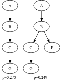
Figure 4: Sample link probability tree and the two causal path instances it generates. Solid, dotted, and dashed arrows indicate ``probably-true,'' ``probably-false,'' and ``try-both'' links, respectively.
(a)
(b)
For each message in the trace, linking attempts to determine if the message is spontaneous or is caused by another message. In many cases, the cause is ambiguous, in which case linking assigns a probability for the link between the parent message into the node and the child message out of the node. The probabilities of the links for all parent messages to a given child message sum to one.
Linking then constructs path instances from these links and
assigns each path instance a confidence score that is the product
of all of the link probabilities in the tree. The total score
across all instances of a given path pattern represents the
algorithm's estimate of the number of times the pattern appeared
in the trace. If a link is sufficiently ambiguous (e.g., if it
has a probability near 0.5), two path instances will be built,
one with the link and one without it. Figure 4 shows an example link probability tree
and the causal path instances it generates. The tree on the left
shows all of the messages that might have been caused, directly
or indirectly, by one specific A![]() B message,
with a probability assigned to each possible link. From this
tree, the linking algorithm generates the two causal path
instances on the right, each with a probability based on the
decisions made to form it. Here, two path instances are generated
because the link between A
B message,
with a probability assigned to each possible link. From this
tree, the linking algorithm generates the two causal path
instances on the right, each with a probability based on the
decisions made to form it. Here, two path instances are generated
because the link between A![]() B and B
B and B![]() F has
probability close to
F has
probability close to ![]() .
.
In broad terms, the linking algorithm consists of three steps: (1) estimating the average causal delay for each node, (2) determining possible parents for each message, and (3) building path instances and then aggregating them into path patterns. We describe the algorithm in more detail in the sections that follow.
The probability of each link between a parent message into B
and a child message out of B is a function of how well it fits
the causal delay distribution. Causal delays represent the
service times at each node. Therefore, as is common in system
modeling, we fit them to an exponential distribution
![]() [16], where
[16], where ![]() is a scaling
parameter to be found. Figure 6 shows a
sample exponential distribution. An exponential distribution
exactly models systems in which service times are
memoryless--that is, the probability that a task will complete in
the next unit time is independent of how long the task has been
running. However, not all systems have memoryless service times.
Even in systems with other service time distributions, the
exponential distribution retains a useful property: because it is
a monotonically decreasing function, the linking algorithm will
assign the highest probability to causal relationships between
messages close to each other in time. Thus, the exponential
distribution works well even if its scaling factor is incorrect
or the system does not exhibit strictly memoryless service
times.
is a scaling
parameter to be found. Figure 6 shows a
sample exponential distribution. An exponential distribution
exactly models systems in which service times are
memoryless--that is, the probability that a task will complete in
the next unit time is independent of how long the task has been
running. However, not all systems have memoryless service times.
Even in systems with other service time distributions, the
exponential distribution retains a useful property: because it is
a monotonically decreasing function, the linking algorithm will
assign the highest probability to causal relationships between
messages close to each other in time. Thus, the exponential
distribution works well even if its scaling factor is incorrect
or the system does not exhibit strictly memoryless service
times.
We also considered
![]() , a gamma
distribution in which
, a gamma
distribution in which ![]() . This gamma distribution assigns the
highest probabilities to delays near
. This gamma distribution assigns the
highest probabilities to delays near ![]() , which
causes the linking algorithm to produce more accurate results if
, which
causes the linking algorithm to produce more accurate results if
![]() is estimated correctly, but much worse results otherwise.
is estimated correctly, but much worse results otherwise.
We use an independent exponential distribution for each
B![]() C pair, by estimating the average delay
C pair, by estimating the average delay
![]() that B waits before sending a
message to C. The delay distribution scaling factor
that B waits before sending a
message to C. The delay distribution scaling factor
![]() is equal to
is equal to
![]() .
.
Correctly determining
![]() requires accurate knowledge of
which message caused which; thus, linking only approximates
requires accurate knowledge of
which message caused which; thus, linking only approximates
![]() and hence
and hence
![]() . Linking estimates
. Linking estimates
![]() as the average of the smallest
delay preceding each message. That is, for each message
B
as the average of the smallest
delay preceding each message. That is, for each message
B![]() C, it finds the latest message into B
that preceded it and includes that delay in the average. If there
is no preceding message within
C, it finds the latest message into B
that preceded it and includes that delay in the average. If there
is no preceding message within ![]() seconds,
B
seconds,
B![]() C is assumed to be a spontaneous
message and no delay is included. The value of
C is assumed to be a spontaneous
message and no delay is included. The value of ![]() should be longer
than the longest real delay in the trace. We use
should be longer
than the longest real delay in the trace. We use ![]() sec for the
Coral and CoDeeN traces, but
sec for the
Coral and CoDeeN traces, but ![]() for the
Slurpee trace. The value of
for the
Slurpee trace. The value of ![]() is user-specified,
depends only on expected processing times, and does not need to
be a tight bound.
is user-specified,
depends only on expected processing times, and does not need to
be a tight bound.
In the presence of high parallelism, the estimate for each
![]() may
be too low, because the true parent message may not be the most
recent one. However, because the exponential distribution is
monotonically decreasing, the ranking of possible parents for a
message is preserved even when
may
be too low, because the true parent message may not be the most
recent one. However, because the exponential distribution is
monotonically decreasing, the ranking of possible parents for a
message is preserved even when ![]() and
and ![]() are wrong. It
is possible to iterate over steps (1) and (2) to improve the
estimate of
are wrong. It
is possible to iterate over steps (1) and (2) to improve the
estimate of ![]() , but linking does not currently do so.
, but linking does not currently do so.
After estimating
![]() for each communicating
pair of nodes B
for each communicating
pair of nodes B![]() C, the linking algorithm assigns each
causal link a weight based on its delay. The weight of the link
between X
C, the linking algorithm assigns each
causal link a weight based on its delay. The weight of the link
between X![]() B and B
B and B![]() C in the
example in Figure 5 is set
to
C in the
example in Figure 5 is set
to
where ![]() is the delay between the arrival of
X
is the delay between the arrival of
X![]() B and the departure B
B and the departure B![]() C.
Additionally, B
C.
Additionally, B![]() C may not have been caused by any
earlier message into B, and instead might have been spontaneous.
This possibility is given a weight equal to a link with delay
C may not have been caused by any
earlier message into B, and instead might have been spontaneous.
This possibility is given a weight equal to a link with delay
![]() .
. ![]() should be a small
constant; we use
should be a small
constant; we use ![]() . A larger
. A larger ![]() instructs the
algorithm to prefer longer paths, while a smaller
instructs the
algorithm to prefer longer paths, while a smaller ![]() generates many short
paths that may be suffixes of correct paths. Spontaneous action
is the most likely choice only when there are no messages into B
within the last
generates many short
paths that may be suffixes of correct paths. Spontaneous action
is the most likely choice only when there are no messages into B
within the last
![]() time. Figure 6 shows the weights assigned to all three possible
parents of B
time. Figure 6 shows the weights assigned to all three possible
parents of B![]() C, as well as the weight assigned to
the possibility that it occurred spontaneously.
C, as well as the weight assigned to
the possibility that it occurred spontaneously.
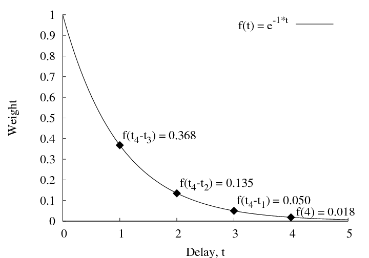
Figure 6: An exponential
distribution with ![]() , showing the weights assigned to all
possible parents of B
, showing the weights assigned to all
possible parents of B![]() C.
C. ![]() represents the
possibility of a spontaneous message, given
represents the
possibility of a spontaneous message, given ![]() .
.
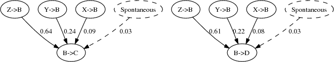
Once all of the possible parents for this B![]() C message
have been enumerated, the weights of their links are normalized
to sum to 1. These normalized weights become the probability for
each link. Figure 7 shows the
possible parents for the B
C message
have been enumerated, the weights of their links are normalized
to sum to 1. These normalized weights become the probability for
each link. Figure 7 shows the
possible parents for the B![]() C and B
C and B![]() D calls,
with their assigned probabilities.
D calls,
with their assigned probabilities.
Hosts or processes that were not traced result in nil
timestamps in the reconciled trace. That is, if node A was traced
and B was not, then A![]() B messages will be present with send
timestamps but not receive timestamps, and B
B messages will be present with send
timestamps but not receive timestamps, and B![]() A messages
will have only receive timestamps. Both estimating
A messages
will have only receive timestamps. Both estimating
![]() and assigning possible parents
to B
and assigning possible parents
to B![]() A rely on having timestamps at both
nodes. In this case, we use A's timestamps in place of B's and
only allow causality back to the same node: A
A rely on having timestamps at both
nodes. In this case, we use A's timestamps in place of B's and
only allow causality back to the same node: A![]() B
B![]() A. This assumption allows calls
from or to nodes outside the traced part of the system but avoids
false causality between, e.g., several unrelated calls to the
same server.
A. This assumption allows calls
from or to nodes outside the traced part of the system but avoids
false causality between, e.g., several unrelated calls to the
same server.
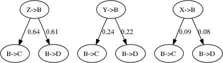
After enumerating and weighting all possible parents for each message, the linking algorithm uses these links to generate a list of the possible children for each message, preserving the link probabilities. This inversion, shown in Figure 8, is necessary because causal path instances are built from the root down.
The final step of the linking algorithm builds path instances from the individual links, then aggregates them into path patterns. That is, if step (2) finds the relationships shown in Figure 4(a), it would generate the two causal path instances shown in Figure 4(b), with the following probabilities:
Each causal link included contributes a factor ![]() corresponding to its
probability. Each causal link omitted contributes a
corresponding to its
probability. Each causal link omitted contributes a ![]() factor.
factor.
For each link in the tree (e.g., did A![]() B cause
B
B cause
B![]() C?), step (3) treats it as
probably-false, probably-true, or try-both, based on its probability. Decisions are
designated try-both if their probability is close to 0.5 or if
they represent one of the most likely causes for a given message.
That is, in Figure 4, if
A
C?), step (3) treats it as
probably-false, probably-true, or try-both, based on its probability. Decisions are
designated try-both if their probability is close to 0.5 or if
they represent one of the most likely causes for a given message.
That is, in Figure 4, if
A![]() B is the most likely cause of
B
B is the most likely cause of
B![]() D, then the A
D, then the A![]() B
B![]() D link will be made a try-both even
though its probability is not near 0.5, ensuring that at least
one cause of B
D link will be made a try-both even
though its probability is not near 0.5, ensuring that at least
one cause of B![]() D is considered even if each possible
cause has probability
D is considered even if each possible
cause has probability ![]() . The number of path instances generated
from a given root message is
. The number of path instances generated
from a given root message is ![]() , where
, where
![]() is
the number of ambiguous links from that message or its
descendants that are treated as try-both. Therefore,
is
the number of ambiguous links from that message or its
descendants that are treated as try-both. Therefore, ![]() must be limited to
bound the running time of linking.
must be limited to
bound the running time of linking.
Linking assigns a probability to each tree equal to the
product of the probabilities of the individual decisions--using
![]() for decisions to omit a causal link--made while constructing it.
If a specific path pattern is seen several times, we keep track
of the total score (i.e., the expected number of times the
pattern was seen) and the maximum probability. Path patterns in
the output are generally ordered by total score.
for decisions to omit a causal link--made while constructing it.
If a specific path pattern is seen several times, we keep track
of the total score (i.e., the expected number of times the
pattern was seen) and the maximum probability. Path patterns in
the output are generally ordered by total score.
Big trees will have low scores because more decisions (more uncertainty) goes into creating them. This behavior is expected.
The latency at each node B is the time between the receive timestamp of the parent message arriving at a node B and the send timestamp of the child message that node B sends. Since both timestamps are local to B, clock offset and clock skew do not affect node latency. For aggregated trees, the linking algorithm calculates the average of that node's delays at each instance of the tree, weighted by the probability of each instance. In addition to the average, we optionally generate a histogram of delays for each node in the tree.
The network latency of each message is the difference between its send and receive timestamps. These timestamps are relative to different clocks (they come from LibSockCap logs at different hosts), so the resulting latency includes clock offset and skew unless we estimate it and subtract it out. We use a filter on the output of the linking algorithm to approximate pairwise clock offset by assuming symmetric network delays, following Paxson's technique [12]. For simplicity, we ignore the effects of clock skew. As a result, our results hide clock offset and exhibit symmetric average delays between pairs of hosts.
Our earlier work, Project 5 [1], presented two causal-path analysis algorithms, nesting and convolution. The nesting algorithm works only on applications using call-return communication and can detect infrequent causal paths (albeit with some inaccuracy as their frequency drops). However, messages must be designated as either calls or returns and paired before running the nesting algorithm. If call-return information is not inherently part of the trace, as in the systems analyzed here, then trying to guess it is error-prone and is a major source of inaccuracy. Linking and nesting both try to infer the cause, if any, for each message or call-return pair in the trace individually.
The nesting algorithm only uses one timestamp per message. It is therefore forced either to ignore clock offset or to use fuzzy timestamp comparisons [1], which only work when all clocks differ by less time than the delays being measured. Since clocks are often unsynchronized--PlanetLab clocks sometimes differ by minutes or hours--our approach of using both send and receive timestamps works better for wide-area traces.
The convolution algorithm uses techniques from signal processing, matching similar timing signals for the messages coming into a node and the messages leaving the same node. Convolution works with any style of message communication, but it requires traces with a minimum of hundreds of messages, runs much more slowly than nesting or linking, and is inherently unable to detect rare paths. When we applied convolution to Coral, it could not detect rare paths like DHT calls and could not separate node processing times of interest from network delays and clock offset.
The linking and nesting algorithms both have ![]() running
time, determined by the need to sort messages in the trace by
timestamp, but both are dominated by an
running
time, determined by the need to sort messages in the trace by
timestamp, but both are dominated by an ![]() component for the
traces we have tried. The convolution algorithm requires
component for the
traces we have tried. The convolution algorithm requires
![]() running time, where
running time, where
![]() is
the duration of the trace and
is
the duration of the trace and ![]() is the size of the
shortest delays of interest. In practice, convolution usually
takes one to four hours to run, nesting rarely takes more than
twenty seconds, and linking takes five to ten minutes but can
take much less or much more given a non-default number of
try-both decisions allowed per causal-link tree. Linking and
nesting both require
is the size of the
shortest delays of interest. In practice, convolution usually
takes one to four hours to run, nesting rarely takes more than
twenty seconds, and linking takes five to ten minutes but can
take much less or much more given a non-default number of
try-both decisions allowed per causal-link tree. Linking and
nesting both require ![]() memory because they load the entire trace into
memory, while convolution requires a constant amount of memory,
typically under 1 MB. Our Project 5 paper [1] has more details for
nesting and convolution, while Section 6 has more details for linking.
memory because they load the entire trace into
memory, while convolution requires a constant amount of memory,
typically under 1 MB. Our Project 5 paper [1] has more details for
nesting and convolution, while Section 6 has more details for linking.
Table 2: Trace statistics
| Trace | Date | Number of messages | Trace duration | Number of hosts |
|---|---|---|---|---|
|
CoDeeN |
Sept. 3, 2004 | 4,702,865 | 1 hour | 115 |
| Coral | Sept. 6, 2004 | 4,246,882 | 1 hour | 68 |
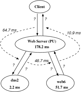
Figure 9: Example of
call-tree visualization.
Solid arrows show message paths, labeled one-way delays, when
known. Dotted arcs show node-internal delays between message
events. Nodes are labeled with name and total delay for node
and its children.
In this section, we present some results from our analyses of traces from the CoDeeN and Coral PlanetLab applications. Table 2 presents some overall statistics for these two traces.
For a given causal path pattern, we use a timeline to represent both causality and time; for example, see Figures 10, 12, 13, and 14. Boxes represent nodes and lines represent communication links; each node or line is labeled with its mean delay in msec. If we do not have traces from a node, we cannot distinguish its internal delay from network delays, so we represent the combination of such a node and its network links as a diamond, labeled with the total delay for that combination. Time and causality flow left to right, so if a node issues an RPC call, it appears twice in the timeline: once when it sends the call, and again when it receives the return.
These timelines differ from the call-tree pictures traditionally used to represent system structure (for example, Figure 1 in [19] and Figure 1 in [7], or the diagrams in our earlier work [1]) but we found it hard to represent both causality and delay in a call-tree, especially when communication does not follow a strict call-return model. Magpie [2] also uses timelines, although Magpie separates threads or nodes vertically, while we only do so when logically parallel behavior requires it.
It is possible to transform the timeline in Figure 10 to a call tree, as in the hand-constructed Figure 9, but this loses the visually helpful proportionality between different delays.
Table 3: Code names for hosts used in figures.
| Code name | Hostname |
|---|---|
| A&M | planetlab2.tamu.edu |
| A&T | CSPlanet2.ncat.edu |
| CMU | planetlab-2.cmcl.cs.cmu.edu |
| CT | planlab2.cs.caltech.edu |
| How | nodeb.howard.edu |
| MIT | planetlab6.csail.mit.edu |
| MU | plnode02.cs.mu.oz.au |
| ND | planetlab2.cse.nd.edu |
| PU | planetlab2.cs.purdue.edu |
| Pri | planetlab-1.cs.princeton.edu |
| Ro | planet2.cs.rochester.edu |
| UCL | planetlab2.info.ucl.ac.be |
| UVA | planetlab1.cs.virginia.edu |
| WaC | cloudburst.uwaterloo.ca (Coral DHT process) |
| WaP | cloudburst.uwaterloo.ca (Proxy process) |
| cl | Any client |
| dns |
some DNS server |
| lo | local loopback |
| web |
some Web origin server |
To avoid unreadably small fonts, we use short code names in the timelines instead of full hostnames. Table 3 provides a translation.
Our tools allow us to characterize and compare causal path patterns. For example, Figure 10 and Figure 12 show, for Coral and CoDeeN respectively, causal path patterns that include a cache miss and a DNS lookup. One can see that CoDeeN differs from Coral in its use of two proxy hops (described in [19] as a way to aggregate requests for a given URL on a single CoDeeN node).
A user of our tools can see how overall system delay is broken down into delays on individual hosts and network links. Further, the user can explore how application structure can affect performance. For example, does the extra proxy hop in CoDeeN contribute significantly to client latency?
Note that we ourselves are not able to compare the end-to-end performance of Coral and CoDeeN because we do not have traces made at clients. For example, one CDN might be able to optimize client network latencies at the cost of poorer server load balancing.
When looking for a performance bug in a replicated distributed system, it can be helpful to look for large differences in delay between paths that should behave similarly. Although we do not believe there were any gross performance problems in either CoDeeN or Coral when our traces were captured, we can find paths with significantly different delays. For example, Figure 13 shows two different but isomorphic cache-miss paths for CoDeeN (these paths do not require DNS lookups). The origin server delay (a total including both network and server delay) is 321 ms in the top path but only 28 ms in the bottom path. Also, the proxies in the top path show larger delays when forwarding requests than those in the bottom path. In both cases, the proxies forward responses rapidly.
Table 4: Examples of mean delays in proxy nodes.
| Node name | Mean delay | Number of samples |
|---|---|---|
| CoDeeN | ||
| planet1.scs.cs.nyu.edu | 0.29 ms | 583 |
| pl1.ece.toronto.edu | 1.47 ms | 266 |
| planlab1.cs.caltech.edu | 0.59 ms | 247 |
| nodeb.howard.edu | 4.86 ms | 238 |
| planetlab-3.cmcl.cs.cmu.edu | 0.20 ms | 53 |
| Coral | ||
| planet1.scs.cs.nyu.edu | 4.84 ms | 6929 |
| planetlab12.Millennium.Berkeley.EDU | 6.16 ms | 3745 |
| planetlab2.csail.mit.edu | 5.51 ms | 1626 |
| CSPlanet2.chen.ncat.edu | 0.98 ms | 987 |
| planetlab14.Millennium.Berkeley.EDU | 0.91 ms | 595 |
Similarly, we can focus on just one role in a path and compare the delays at the different servers that fill this role. Table 4 shows mean delays in proxies for cache-hit operations (the causal path patterns in this case are trivial).
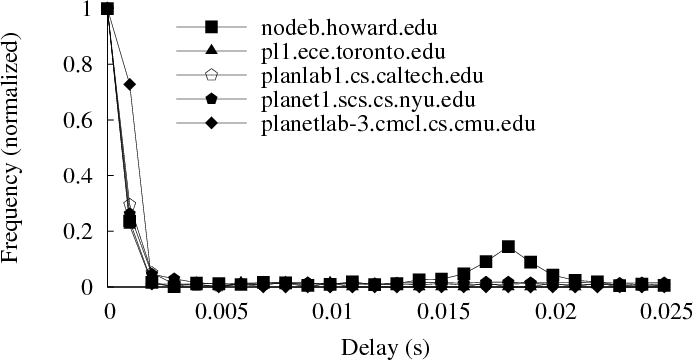
The message linking algorithm has enough information to generate the entire distribution of delays at a node or on a link rather than just the mean delay. Figure 11 shows the delay distributions for cache-hit operations on five nodes. The nodes in this figure are also listed in Table 4, which shows mean delay values for four of the nodes between 0 and 2 ms. The distribution for nodeb.howard.edu shows two peaks, including one at 18 ms that strongly implies a disk operation and corresponds with this node's higher mean delay in the table.
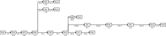
Coral uses a distributed hash table (DHT) to store information about which proxy nodes have a given URL and to store location information about clients.1 Whenever a proxy does not have a requested web object in its local cache, it searches the DHT to find other nodes that have the object, and it inserts a record into the DHT once it has retrieved the object. Figure 14 shows one such DHT call in Coral. The sets of three parallel calls in this figure reflect Coral's use of three overlapping DHTs at different levels of locality. From the figure, it is also clear that Coral's DHT is iterative: each hop in a DHT path responds directly to the requester rather than forwarding the query to the next hop.
Table 5: Runtime costs for analyzing several traces
| Trace | Number of messages | Trace duration | Reconciliation | Message Linking | ||
|---|---|---|---|---|---|---|
| CPU secs | MBytes | CPU secs | MBytes | |||
| CoDeeN | 4,702,865 | 1 hours | 982 | 697 | 730 | 1354 |
| Coral | 4,246,882 | 1 hours | 660 | 142 | 517 | 1148 |
We measured the CPU time and memory required to run the
reconciliation and message linking algorithms on several traces.
Table 5 shows that these costs are
acceptable. The CPU time requirements are higher than the nesting
algorithm but lower than the convolution algorithm [1]. The memory requirements
reflect the need to keep the entire trace in memory for both
reconciliation and linking. We expect the running time to be
![]() for both reconciliation and linking
because both require sorting. However, the
for both reconciliation and linking
because both require sorting. However, the ![]() portions of each
program dominate the running time. The running time for linking
is heavily dependent on the pruning parameters used, particularly
the number of try-both bits allocated per link probability tree.
Memory requirements are
portions of each
program dominate the running time. The running time for linking
is heavily dependent on the pruning parameters used, particularly
the number of try-both bits allocated per link probability tree.
Memory requirements are ![]() for both
programs.
for both
programs.
The linking algorithm produces two scores for each path pattern it identifies: a raw count of the number of instances and expected number of instances believed to be real. The latter is the sum of the probabilities of all instances of the path pattern. Sorting by the expected number of instances is generally the most useful, in that the patterns at the top of the list appear many times, have high confidence, or both. Highlighting paths that appear many times is useful because they are where optimizations are likely to be useful. Highlighting paths with high confidence helps suppress false positives (i.e., patterns that are inferred but do not reflect actual program behavior).
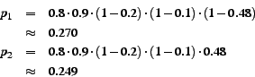
Two additional, composite metrics are: (1)
![]() and (2)
and (2)
![]() . The first is the
average probability of instances of each path, and it favors
high-confidence paths. The second captures the notion that seeing
a path many times increases the confidence that it is not a false
positive, but not linearly.
. The first is the
average probability of instances of each path, and it favors
high-confidence paths. The second captures the notion that seeing
a path many times increases the confidence that it is not a false
positive, but not linearly.
Although this paper focuses on wide-area applications, previous work on black-box debugging using traces [1,2,4] focused on LAN applications. We had the opportunity to try our tools on traces from a moderately complex enterprise application, Slurpee2. We do not present detailed results from Slurpee, since LAN applications are not the focus of the paper and space does not permit an adequate treatment. However, Slurpee is the one system on which we have used linking, nesting, and convolution. Further, we learned several things applying WAP5 to Slurpee that are applicable to wide-area applications.
The Slurpee system aids in supporting customers of a computer vendor. It handles reports of incidents (failures or potential failures) and configuration changes. Reports arrive via the Internet, and are passed through several tiers of replicated servers. Between each tier there are firewalls, load balancers, and/or network switches as appropriate, which means that the component servers are connected to a variety of distinct LANs.
Since we could not install LibSockCap on the Slurpee servers, packet-sniffing was our only option for tracing Slurpee and had the advantage of non-invasiveness. However, we found the logistics significantly more daunting than we expected. Packet sniffing systems are expensive, and we could not allocate enough of them to cover all packet paths. They also require on-site staff support to set them up, configure switch ports, initiate traces, and collect the results. In the future, these tasks might be more automated.
We obtained simultaneous packet traces from five sniffers, one for each of the main LAN segments behind the main firewall. We treated each packet as a message, and applied a variant of our reconciliation algorithm (see Section 4) to generate a unified trace.
The five sniffers did not have synchronized clocks when the traces were made. Clock offsets were on the order of a few seconds. Since we had two copies of many packets (one sniffed near the sender, one sniffed near the receiver), we developed an algorithm to identify which sniffer's clock to use as the sender or receiver timestamp for each server (node) in the trace. If the sniffer is on the same switch as a node, then every packet to or from that node appears in that sniffer's traces. If we did not sniff the node's switch, then we chose the sniffer that contained the most packets to or from the node.
We applied all three of our causal-path analysis algorithms to the Slurpee trace. The Slurpee trace conforms to call-return semantics but does not contain the information needed to pair calls with returns. We tried several heuristics for pairing calls and returns, but the inaccuracy in this step limited the usefulness of the nesting algorithm. Convolution does not require call-return pairing, but it does require a large number of instances of any given path. Several of the Slurpee paths occurred infrequently and were not detected by convolution. Some of the Slurpee hosts were only visible in the trace for a few seconds and so did not send or receive enough messages to appear in any path detected by convolution. Linking was able to detect both common and rare paths and was not hampered by the lack of call-return pairing information.
In analyzing the Slurpee system, we found instances of network address translation, which did not appear in the Coral or CoDeeN traces but which might appear in other wide-area systems.
Network address translation (NAT) [6] allows network elements to change the addresses in the packets they handle. In Slurpee, a load balancer uses NAT to redirect requests to several server replicas. Wide-area systems often use NAT to reduce the pressure on IPv4 address space assignments. NAT presents a problem for message-based causality analysis, because the sender and receiver of a single message use different ``names'' (IP addresses) for one of the endpoints.
We developed a tool to detect NAT in packet traces and to rewrite trace records to canonicalize the translated addresses. This tool searches across a set of traces for pairs of packets that have identical bodies and header fields, except for IP addresses and headers that normally change as the result of routing or NAT. While small numbers of matches might be accidental (especially for UDP packets, which lack TCP's pseudo-random sequence numbers), frequent matches imply the use of NAT. The tool can also infer the direction of packet flow using the IP header's Time-To-Live (TTL) field, and from packet timestamps if we can correct sufficiently for clock offsets.
We have not tested this tool on packet traces from a wide-area system, but we believe it would work correctly. However, because LibSockCap does not capture message contents and cannot capture packet headers, LibSockCap traces do not currently contain enough information to support this tool.
We divide related work into three categories: trace-based techniques for causality and performance analysis, and other interposition-based tools.
Our previous work on Project 5 [1], which we have already described earlier in this paper, is most closely related work to WAP5. This earlier work ignored many practical issues in gathering traces, particularly overlapping traces from multiple sniffers, and reconciling them into a single trace for analysis. Also, Project 5's nesting algorithm depends on call-return semantics and is too sensitive to clock offsets, while the convolution algorithm requires long traces and cannot infer causality in the presence of highly variable processing delays.
Magpie [2] complements our work by providing a very detailed picture of what is happening at each machine, at the cost of needing to understand the applications running at each machine. Magpie uses Event Tracing for Windows, built into the Windows operating system, to collect thread-level CPU and disk usage information. Magpie does not require modifying the application, but does require ``wrappers'' around some parts of the application. Their algorithms also require an application-specific event schema, written by an application expert, to stitch traced information into request patterns.
Several other systems require instrumented middleware or binaries. Pinpoint [4] focuses on finding faults by inferring them from anomalous behavior. Pinpoint instruments the middleware on which an application runs (e.g., J2EE) in order to tag each call with a request ID. The Distributed Programs Monitor (DPM) [10] instruments a platform to trace unmodified applications. DPM uses kernel instrumentation to track the causality between pairs of messages rather than inferring causality from timestamps. Paradyn [11] uses dynamic instrumentation to capture events and location bottlenecks, but it does not organize events into causal paths. Finally, some of the most invasive systems, such as NetLogger [14] and ETE [8], find causal paths in distributed system by relying on programmers to instrument interesting events rather than inferring them from passive traces. Pip [13] requires modifying, or at least recompiling, applications but can extract causal path information with no false positives or false negatives. Because of the higher information accuracy, Pip can check the extracted behavior against programmer-written templates and identify any unexpected behavior as possible correctness or performance bugs.
Several other systems use interposition. Trickle [15] uses library interposition to provide user-level bandwidth limiting. ModelNet [18] rewrites network traffic using library interposition to multiplex emulated addresses on a single physical host. Systems such as Transparent Result Caching [17] and Interposition Agents [9] used debugging interfaces such as ptrace or /proc to intercept system calls instead of library interposition. Library interposition is simpler and more efficient, but it requires either dynamically linked binaries or explicit relinking of traced applications.
We have developed a set of tools called Wide-Area Project 5 (WAP5) that helps expose causal structure and timing in wide-area distributed systems. Our tools include a tracing infrastructure, which includes a network interposition library called LibSockCap and algorithms to reconcile many traces into a unified list of messages; a message-linking algorithm for inferring causal relationships between messages; and visualization tools for generating timelines and causal trees. We applied WAP5 to two content-distribution networks in PlanetLab, Coral and CoDeeN, and to an enterprise-scale incident-monitoring system, Slurpee. We extracted a causal behavior model from each system that matched published descriptions (or, for Slurpee, our discussions with the maintainers). In addition, we were able to examine the performance of individual nodes and the hop-by-hop components of delay for each request.
[1] M. K. Aguilera, J. C. Mogul, J. L. Wiener, P. Reynolds, and A. Muthitacharoen. Performance debugging for distributed systems of black boxes. In Proc. SOSP-19, Bolton Landing, NY, Oct. 2003.
[2] P. Barham, A. Donnelly, R. Isaacs, and R. Mortier. Using Magpie for request extraction and workload modelling. In Proc. 6th OSDI, San Francisco, CA, Dec. 2004.
[3] A. Bavier, M. Bowman, B. Chun, D. Culler, S. Karlin, S. Muir, L. Peterson, T. Roscoe, T. Spalink, and M. Wawrzoniak. Operating System Support for Planetary-Scale Services. In Proc. NSDI, pages 253-266, Mar. 2004.
[4] M. Chen, A. Accardi, E. Kiciman, J. Lloyd, D. Patterson, A. Fox, and E. Brewer. Path-based failure and evolution management. In Proc. NSDI, pages 309-322, San Francisco, CA, Apr. 2004.
[5] F. Dabek, J. Li, E. Sit, J. Robertson, M. F. Kaashoek, and R. Morris. Designing a DHT for Low Latency and High Throughput. In Proc. NSDI, pages 85-98, Mar. 2004.
[6] K. B. Egevang and P. Francis. The IP Network Address Translator (NAT). RFC 1631, IETF, May 1994.
[7] M. J. Freedman, E. Freudenthal, and D. Mazičres. Democratizing Content Publication with Coral. In Proc. NSDI, pages 239-252, San Francisco, CA, Mar. 2004.
[8] J. L. Hellerstein, M. Maccabee, W. N. Mills, and J. J. Turek. ETE: A customizable approach to measuring end-to-end response times and their components in distributed systems. In Proc. ICDCS, pages 152-162, Austin, TX, May 1999.
[9] M. B. Jones. Interposition agents: Transparently interposing user code at the system interface. In Proc. SOSP-14, pages 80-93, Asheville, NC, Dec. 1993.
[10] B. P. Miller. DPM: A Measurement System for Distributed Programs. IEEE Trans. on Computers, 37(2):243-248, Feb 1988.
[11] B. P. Miller, M. D. Callaghan, J. M. Cargille, J. K. Hollingsworth, R. B. Irvin, K. L. Karavanic, K. Kunchithapadam, and T. Newhall. The Paradyn Parallel Performance Measurement Tool. IEEE Computer, 28(11):37-46, Nov. 1995.
[12] V. Paxson. On calibrating measurements of packet transit times. In Proc. SIGMETRICS, Madison, WI, Mar. 1998.
[13] P. Reynolds, C. Killian, J. L. Wiener, J. C. Mogul, M. A. Shah, and A. Vahdat. Pip: Detecting the unexpected in distributed systems. In Proc. NSDI, San Jose, CA, May 2006.
[14] B. Tierney, W. Johnston, B. Crowley, G. Hoo, C. Brooks, and D. Gunter. The NetLogger methodology for high performance distributed systems performance analysis. In Proc. IEEE High Performance Distributed Computing Conf. (HPDC-7), July 1998.
[15] Trickle lightweight userspace bandwidth shaper. http:/monkey.org/~marius/trickle/.
[16] K. S. Trivedi. Probability and Statistics with Reliability, Queueing, and Computer Science Applications. John Wiley and Sons, New York, 2001.
[17] A. Vahdat and T. Anderson. Transparent result caching. In Proc. USENIX Annual Tech. Conf., June 1998.
[18] A. Vahdat, K. Yocum, K. Walsh, P. Mahadevan, D. Kostic, J. Chase, and D. Becker. Scalability and Accuracy in a Large-Scale Network Emulator. In Proc. 5th OSDI, 2002.
[19] L. Wang, K. Park, R. Pang, V. Pai, and L. Peterson. Reliability and Security in the CoDeeN Content Distribution Network. In Proc. USENIX 2004 Annual Tech. Conf., pages 171-184, Boston, MA, June 2004.
[20] M. Welsh, D. Culler, and E. Brewer. Seda: an architecture for well-conditioned, scalable internet services. In Proc. 18th SOSP, pages 230-243, 2001.