 |
 |
|
I(P) = IB(P); G = 100
|
|
Department of Computer Science
Stanford University, CA 94305, U.S.A.
cho@cs.stanford.edu,
hector@cs.stanford.edu and
page@cs.stanford.edu
A crawler is a program that retrieves Web pages, commonly for use by a search engine [Pinkerton 1994]. Roughly, a crawler starts off with the URL for an initial page P0. It retrieves P0, extracts any URLs in it, and adds them to a queue of URLs to be scanned. Then the crawler gets URLs from the queue (in some order), and repeats the process.
Crawlers are widely used today. Crawlers for the major search engines (e.g., Altavista [1], and Excite [2]) attempt to visit most text Web pages, in order to build content indexes. At the other end of the spectrum, we have personal crawlers that scan for pages of interest to a particular user, in order to build a fast access cache (e.g. NetAttache [3])
The design of a good crawler presents many challenges. Externally, the crawler must avoid overloading Web sites or network links as it goes about its business [Koster 1995]. Internally, the crawler must deal with huge volumes of data. Unless it has unlimited resources and time, it must carefully decide what URLs to scan and in what order. The crawler must also decide how frequently to revisit pages it has already seen, in order to keep its client informed of changes on the Web.
In this paper we address one of these important challenges: How should a crawler select URLs to scan from its queue of known URLs? If a crawler intends to perform a single scan of the entire Web, then any URL order will suffice. That is, eventually every single known URL will be visited, so the order is not critical. However, most crawlers will not be able to visit every possible page for two main reasons:
In either case, it is important for the crawler to visit "important" pages first, so that the fraction of the Web that is visited is more meaningful. In this paper we present several useful definitions of importance, and develop crawling priorities so that important pages have a higher probability of being visited first. We also present experimental results from crawling the Stanford University Web pages that show how effective the different crawling strategies are. (An extended version of this paper, with additional results, can be found at http://www-db.stanford.edu/~cho/crawler-paper/complete-paper.html.)
Of course, a crawler must also avoid overloading target sites' important pages. In this paper we do not address this issue. That is, we assume that URLs selected for scanning may be delayed by a crawler component that monitors site loads, but we do not study here how this delay component works. Similarly, we do not consider in this paper rescanning pages. In practice one may of course wish to start rescanning important pages even before a crawl is completed, but this is beyond the scope of this paper.
Not all pages are of equal interest to the crawler's client. For instance, if the client is building a specialized database on a particular topic, then pages that refer to that topic are more important, and should be visited as early as possible. Similarly, a search engine may use the number of Web URLs that point to a page, the so-called backlink count, to rank user query results.
Given a Web page P, we can define the importance of the page, I(P), in one of the following ways (These metrics can be combined, as will be discussed later.):
To compute similarities, we can view each document (P or Q) as an m-dimensional vector <w1, ..., wn>. The term wi in this vector represents the significance of the ith word in the vocabulary. One common way to compute the significance wi is to multiply the number of times the ith word appears in the document by the inverse document frequency (idf) of the ith word. The idf factor is one divided by the number of times the word appears in the entire "document collection". The similarity between P and Q can then be defined as the inner product of the P and Q vectors.
Note that if we use idf terms in our similarity computation, we need global information to compute the importance of a page. During the crawling process we have not seen the entire collection, so we have to estimate the idf factors. We use IS'(P) to refer to the estimated importance of page P, which is different from the actual importance IS(P).If idf factors are not used, then IS'(P) = IS(P).
Note that evaluating IB(P) requires counting backlinks over the entire Web. A crawler may estimate this value with IB'(P), the number of links to P that have been seen so far.
More formally, if a page
has no outgoing link, we assume that it has outgoing links to every single
Web page. Next, consider a page P that is pointed at by pages
T1, ..., Tn. Let ci be
the number of links going out of page Ti. Also, let
d be a damping factor (whose intuition is given below). Then, the
weighted backlink count of page P is given by
IR(P) = (1 – d) + d ( IR(T1)/c1 + ... +
IR(Tn)/cn)
This leads to one equation per
Web page, with an equal number of unknowns. The equations can be solved
for the IR values. They can be solved iteratively, starting with
all IR values equal to 1. At each step, the new IR(P) value
is computed from the old IR(Ti) values (using the
equation above), until the values converge.
One intuitive model for PageRank is that we can think of a user "surfing" the Web, starting from any page, and randomly selecting from that page a link to follow. When the user reaches a page with no outlinks, he jumps to a random page. Also, when the user is on a page, there is some probability, d, that the next visited page will be completely random. The IR(P) values we computed above give us the probability that our random surfer is at P at any given time.
Our goal is to design a crawler that if possible visits high I(P) pages before lower ranked ones, for some definition of I(P). Of course, the crawler will only have available I'(P) values, so based on these it will have to guess what are the high I(P) pages to fetch next.
Our general goal can be stated more precisely in three ways, depending on how we expect the crawler to operate. (In our evaluations of Sections 6 and 7 we use the second model in most cases, but we do compare it against the first model in one experiment. Nevertheless, we believe it is useful to discuss all three models to understand the options.)
Crawl & Stop. Under this model, the crawler C starts at its initial page P0 and stops after visiting K pages. At this point a perfect crawler would have visited pages R1, ..., RK, where R1 is the page with the highest importance value, R2 is the next highest, and so on. We call pages R1 through RK the hot pages. The K pages visited by our real crawler will contain only M pages with rank higher than or equal to I(RK). We define the performance of the crawler C to be PCS(C) = (M·100)/K. The performance of the ideal crawler is of course 100%. A crawler that somehow manages to visit pages entirely at random would have a performance of (K·100)/T, where T is the total number of pages in the Web.
Crawl & Stop with Threshold. We again assume that the crawler visits K pages. However, we are now given an importance target G, and any page with I(P) >= G is considered hot. Let us assume that the total number of hot pages is H. The performance of the crawler, PST(C), is the percentage of the H hot pages that have been visited when the crawler stops. If K < H , then an ideal crawler will have performance (K·100)/H. If K >= H, then the ideal crawler has 100% performance. A purely random crawler that revisits pages is expected to visit (H/T) ·K hot pages when it stops. Thus, its performance is (K·100)/T.
Limited Buffer Crawl. In this model we consider the impact of limited storage on the crawling process. We assume that the crawler can only keep B pages in its buffer. Thus, after the buffer fills up, the crawler must decide what pages to flush to make room for new pages. An ideal crawler could simply drop the pages with lowest I(P) value, but a real crawler must guess which of the pages in its buffer will eventually have low I(P) values. We allow the crawler to visit a total of T pages, equal to the total number of Web pages. At the end of this process, the percentage of the B buffer pages that are hot gives us the performance PBC(C). The performances of an ideal and a random crawler are analogous to those in the previous cases.
Note that to evaluate a crawler under any of these metrics, we need to compute the actual I(P) values of pages, and this involves crawling the "entire" Web. To keep our experiments (Section 6 and 7) manageable, we define the entire Web to be the Stanford University pages, and we only evaluate performance in this context. In Section 6 we study the implications of this assumption by also analyzing a smaller Web within the Stanford domain, and seeing how Web size impacts performance.
A crawler keeps a queue of URLs it has seen during the crawl, and must select from this queue the next URL to visit. The ordering metric O is used by the crawler for this selection, i.e., it selects the URL u such that O(u) has the highest value among all URLs in the queue. The O metric can only use information seen (and remembered if space is limited) by the crawler.
In our experiments, we explore the types of ordering metrics that are best suited for either IB(P) or IR(P). For similarity IS(P) metrics, it is hard to devise an ordering metric since we have not seen P yet. As we will see, for similarity, we may be able to use the text that anchors the URL u as a predictor of the text that P might contain.
To avoid network congestion and heavy loads on the servers, we did our experimental evaluation in two steps. In the first step, we physically crawled all Stanford Web pages and built a local repository of the pages. After we built the repository, we ran our virtual crawlers on it to evaluate the different crawling schemes. Note that even though we had the complete image of the Stanford domain in the repository, our virtual crawler based its crawling decisions only on the pages it saw for itself. In this section we briefly discuss how the WebBase crawler operates, and how the particular database was obtained for our experiments.
The actual data the system is allowed to get is reduced for two reasons. The first is that many heuristics are needed to avoid automatically generated, and potentially infinite, sets of pages. For example, any URLs containing "/cgi-bin/" are not crawled. Several other heuristics based on the Location Metric described above are used to weed out URLs which look undesirable.
To download an image of the Stanford Web pages, we started WebBase with an initial list of "stanford.edu" URLs. These 89,119 URLs were obtained from an earlier crawl. During the crawl, non-Stanford URLs were ignored. At the end of the process, we had 784,592 known URLs to Stanford pages. Even though the crawl was stopped before it was complete, most of the uncrawled URLs were on only a few servers so we believe the dataset we used to be a reasonable representation of the stanford.edu Web. This dataset consisted of about 225,000 crawled valid HTML pages.
We should stress that the virtual crawlers that will be discussed next do not use WebBase directly. As stated earlier, they use the dataset collected by the WebBase crawler, and do their own crawling on it. The virtual crawlers are simpler than the Web Base crawler. For instance, they do not need to distribute the load to visited sites. This kind of simplification is fine, since the virtual crawlers are only used to evaluate ordering schemes, and not to do real crawling.
In this section we study the effectiveness of various ordering metrics, for the scenario where importance is measured through backlinks (i.e., either the IB(P) or IR(P) metrics). We start by describing the structure of the virtual crawler, and then consider the different ordering metrics. Unless otherwise noted, we use the Stanford dataset described in Section 5, and all crawls are started from the Stanford homepage [4]. For the PageRank metric we use a damping factor d of 0.9 (for both IR(P) and IR'(P)), for all of our experiments (including those of the following section).
Figure 1 shows our basic virtual crawler. The crawler manages three
main data structures. Queue url_queue
contains the URLs that have been seen and need to be visited. Once a page
is visited, it is stored (with its URL ) in crawled_pages. Finally, links
holds pairs of the form (u1, u2), where URL
u2 was seen in the visited page with URL
u1. The crawler's ordering metric is implemented by
the function, reorder_queue(), shown in
Fig. 2. We used three ordering metrics: (1) breadth-first (2) backlink
count, IB'(P), and (3) PageRank, IR'(P). The breadth-first
metric places URLs in the queue in the order in which they are discovered,
and this makes the crawler visit pages in breadth-first order.
| ||||||||||||||||||||||||||||||||||||||||||||||||||||||||||||||||||||||||||||||||||
| ||||||||||||||||||||||||||||||||||||||||||||||||||||||||||||||||||||||||||||||||
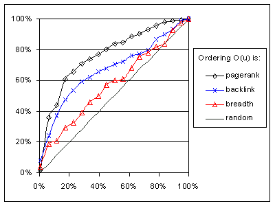
We start by comparing three different ordering metrics, breadth-first, backlink-count, and PageRank (corresponding to the three functions of Fig. 2) in Graph 1. In this scenario, the importance metric is the number of backlinks (I(P) = IB(P)), and we consider a Crawl & Stop with Threshold model (Section 3) with G = 100. (Recall that a page with G or more backlinks is considered important, i.e., hot.) Under this definition, 1,400 (0.8%) pages out of 179,000 valid pages were considered hot. (Out of 225,000 page dataset mentioned in Section 5, 46,000 pages were unreachable from the Stanford homepage. So the total number of pages for the experiment is 179,000 pages.)
In Graph 1, the horizontal axis is the percentage of the dataset that has been crawled over time. At the 100% mark, all 179,000 pages have been visited. For each visited fraction we report on the vertical axis PST, the percentage of the total hot pages that has been visited so far. Graph 1 also shows the performance of a random crawler. As discussed in Section 3, the performance of a random crawler is a straight diagonal line. An ideal crawler (not shown) would reach 100% performance when H pages have been crawled.
 |
 |
|
I(P) = IB(P); G = 100
|
|
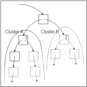
The results are rather counter-intuitive. That is, intuitively one would expect that a crawler using an ordering metric IB'(P) that matches the importance metric IB(P) would perform the best. However, this is not the case, and the IR'(P) metric outperforms the IB'(P) one. To understand why, we manually traced the crawler's operation. We noticed that often the IB'(P) crawler behaved like a depth-first one, frequently visiting pages in one "cluster" before moving on to the next. On the other hand, the IR'(P) crawler combined breadth and depth in a better way. To illustrate consider the Web fragment of Fig. 3.
With IB'(P) ordering, the crawler visits a page like the one labeled 1 and quickly finds a cluster A of pages that point to each other. The A pages temporarily have more backlinks than page 2, so the visit of page 2 is delayed. However, since the whole Web has not been crawled, it may be that page 2 has more backlinks than the A pages. On the other hand, with IR'(P) ordering, page 2 may have higher rank (because its link comes from a high ranking page) than the pages in cluster A (that only have pointers from low ranking pages within the cluster). Therefore, page 2 is reached faster.
In summary, during the early stages of a crawl, the backlink information is biased by the starting point. If the crawler bases its decisions on this skewed information, it tries getting locally hot pages instead of globally hot pages, and this bias gets worse as the crawl proceeds. On the other hand, the IR'(P) PageRank crawler is not as biased towards locally hot pages, so it gives better results regardless of the starting point.
Graph 2 shows the performance PCS of the crawlers under the Crawl & Stop model. The setting is the same as for Graph 1. Keep in mind that an ideal crawler would now have 100% performance at all times. The results are analogous to those of the Crawl & Stop with Threshold model. The key difference is that the PCS results are not dependent on a G value. Thus, the metric PCS may be appropriate if we do not have a predefined notion of what constitutes a hot page.
Returning to the Crawl & Stop with Threshold model, Graph 3 shows the results of using the IR(P) PageRank importance metric. The results are similar to those of Graph 1, except that the IR'(P) is even more effective now.
 |
 |
|
I(P) = IB(P) |
I(P) = IR(P); G = 13
|
As discussed in Section 1, in some cases the crawler's client may only be interested in small portions of the Web. For instance, the client may be interested in a single site (to create a mirror, say). In our next experiment we evaluate the ordering metrics in such a scenario. The results will also let us study the impact of the differences in scale.
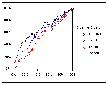
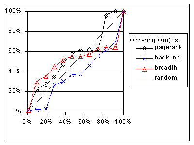
For this experiment we only crawled the pages of the Stanford Database Group (on server www-db.stanford.edu [5]). This subset of the Stanford pages consists of about 1,100 valid HTML pages. In general, crawling performance is not as good on the smaller subset. Graph 4 shows one representative result. In this case, we use the Crawl & Stop with Threshold model with G = 5. The importance metric is IB(P). The graph shows that performance can be even worse than that of a random crawler at times, for all ordering metrics.
|
 |
|
I(P) = IB(P); G = 5. |
(within DB group). |
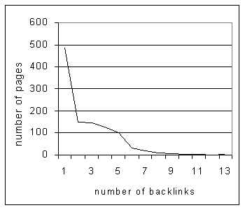
The reason for this poor performance is that IB(P) is not a good importance metric for a small domain. To see this, Graph 5 shows the histogram for the number of backlinks, in our sample domain. The vertical axis shows the number of pages for each backlink count. From this histogram we can see that most pages have fewer than 10 backlinks. In this range, the rank of each page varies greatly according to the style used by the creator of the Web pages. For instance, if the creator generates many cross links between his pages, then his pages have a high IB(P) rank, otherwise they do not. If the high rank pages do not have many links from outside the cluster created by this person, it will be hard to find them. In any case, the rank is not a good measure of the global importance of the pages.
In Graph 4 we can see the impact of "locally dense" clusters. The performance of the backlink IB'(P) crawler is initially quite flat. This is because it initially does a depth-first crawl for the first cluster it found. After visiting about 20% of the pages, the crawler suddenly discovers a large cluster, and this accounts for the jump in the graph there. On the other hand, the PageRank IR'(P) crawler found this large cluster earlier, so its performance is much better initially.
In the experiments of Section 6, we compared three different backlink-based crawlers. In this section, we present the results of our experiments on similarity-based crawlers. The similarity-based importance metric, IS(P), measures the relevance of each page to a topic or a query that the user has in mind. There are clearly many possible IS(P) metrics to consider, so our experiments here are not intended to be comprehensive. Instead, our goal is to briefly explore the potential of various ordering schemes in some sample scenarios. In particular, for our first three experiments we consider the following IS(P) definition: A page is considered hot if it contains the word computer in its title or if it has more th an 10 occurrences of computer in its body.
| ||||||||||||||||||||||||||||||||||||||||||||||||||||||||||||||||||||||||||||||||||||||||||||||||||||||||||||||||||||||||||||||||||||
For similarity-based crawling,
the crawler of Fig. 1 is not appropriate, since it does not take the
content of the page into account. To give priority to the pages mentioning
computer, we modified our crawler as shown in Fig. 4. This
crawler keeps two queues of URLs to visit: hot_queue stores the URLs that have been seen in an anchor
mentioning the word computer, or that have the word computer
within them. The second queue, url_queue,
keeps the rest of the URLs. The crawler first takes URL to visit from
hot_queue.
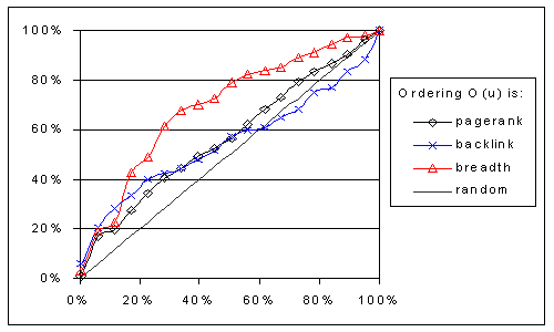
Graph 6 shows the PST results for this crawler, for the IS(P) importance metric defined above. The results show that the backlink-count and the PageRank crawler behaved no better than a random crawler. Only the breadth-first crawler gave a reasonable result. This is a rather unexpected result. That is, all these crawlers differ only in their ordering metrics, which are neutral to the page content. All crawlers visited computer-related URLs immediately after their discovery. Therefore, all the schemes are theoretically equivalent and should give comparable results.
The observed unexpected performance difference arises mainly from the breadth-first crawler's FIFO nature. The breadth-first crawler fetches the pages in the order they are found. If a computer-related page is crawled earlier, then the crawler discovers and visits its child pages earlier as well. These pages have a tendency to also be computer related, so performance is better. Thus, the observed property is that if a page has a high IS(P) value, then its children are likely to have a higher IS(P) value too. Another reason for this difference is that more than a third of the hot pages have only one backlink to them. If the anchors of these pages do not contain the word computer and if they are far from hot pages, their crawling is delayed. Of course, it is questionable if these pages are actually important, since nobody has pointed to them.
To take advantage of the first property, we modified our crawler as shown in Fig. 5. This crawler places in thehot_queue URLs
that have the target keyword in their anchor or within, or that are within
3 links from a hot page.
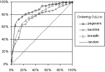
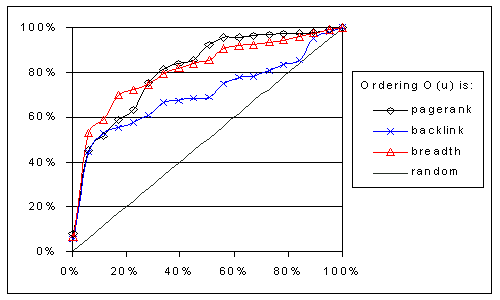
We also modified importance metric so that it takes into account similarity and backlink information. Under our new definition, a page is hot if it is on the computer topic (its title contains computer or its body has 10 or more occurrences of computer) and it has five or more backlinks. Graph 7 shows the PST results for this combined IS(P) and IB(P) importance metric. All crawlers showed significant improvement now. Especially the results of the crawlers that order based on PageRank IR'(P) and breadth-first order are very good. For instance, after having seen only 40% of the pages, these crawlers have obtained over 80% of the hot pages. After visiting 60% of the pages, most of the hot pages have been gathered.
We repeated a similar experiment with a different query topic, admission. The performance details varied from the previous case, but the overall conclusion was the same: When both similarity and the number of backlinks are important, it is effective to use a combined ordering metric that considers IR'(P), the content of anchors, and the distance to pages known to be hot.
| ||||||||||||||||||||||||||||||||||||||||||||||||||||||||||||||||||||||||||||||||||||||||||||||||||||||||||||||||||||||||||||||||||||||||||||||||||||||||||||||||||
In this paper we addressed the problem of ordering URLs for crawling. We listed different kinds of importance metrics, and built three models to evaluate crawlers. We experimentally evaluated several combinations of importance and ordering metrics, using the Stanford Web pages.
In general our results show that PageRank, IR'(P), is an excellent ordering metric when either pages with many backlinks or with high PageRank are sought. In addition, if the similarity to a driving query is important, then it is also useful to visit earlier URLs that:
With a good ordering strategy, it seems to be possible to build crawlers that can rather quickly obtain a significant portion of the hot pages. This can be extremely useful when we are trying to crawl large portions of the Web, when our resources are limited, or when we need to revisit pages often to detect changes.
One limitation of our work is that it only used the Stanford Web pages. We believe that the Stanford pages are a representative sample: For example, they are managed by many different people, who structure their pages in a variety of ways. They include many individual homepages, and also many clusters that are carefully managed by organizations. Nevertheless, in the future we plan to investigate non-Stanford Web pages to analyze structural differences and their implication for crawling.