Rakesh
Agrawal and
Ramakrishnan
Srikant
IBM Almaden Research Center
650 Harry Road, San Jose, CA 95120
Note: We strongly recommend printing the PDF version of this paper.
Copyright is held by the author/owner(s).
WWW2002, May 7-11, 2002, Honolulu, Hawaii, USA.
ACM 1-58113-449-5/02/0005.
'o dear ophelia, I am ill at these numbers; Hamlet: II, iiNumbers play a central role in modern life. Yet the current search engines treat numbers as strings, ignoring their numeric values. For example, as of this writing, the search for 6798.32 on Google yielded two pages that correctly associate this number with the lunar nutation cycle [18]. However, the search for 6798.320 on Google found no page. The search for 6798.320 on AltaVista, AOL, HotBot, Lycos, MSN, Netscape, Overture, and Yahoo! also did not find any page about the lunar nutation cycle.
A large fraction of the useful web comprises of what
can be called specification documents.
They largely consist of attribute-value pairs surrounded with text.
Examples of such documents include product information,
classified advertisements, resumes, etc.
For instance, Figure 1 shows a partial extract
of the data sheet for the Cypress CY7C225A PROM.
A design engineer should be able to ask a query that looks something like this:
address set-up speed 20 ns power 500 mW CMOS PROM
and get the CY7C225A data sheet.
None of the search engines
could find this datasheet using the above query
(or its variations).
We were able to get the data sheet when we provided the exact numeric
values for the speed and power attributes
because the search engines could then match the string.
It is unreasonable to expect that the user will provide exact numeric values
when doing such searches.
In fact, users typically search for items whose specifications roughly
match the values provided in the query.
|
The approach taken in the past to retrieve the specification documents has been to extract the attribute-value pairs contained in a document and store them in a database. Queries can now be answered using nearest neighbor techniques [1] [15] [21]. There has been some research on automating the task of data extraction (see surveys in [7] [19]). However, the automatic extraction of attribute-value pairs has a spotty record of success. It is a hard problem, exacerbated by the fact that it is often difficult to identify attribute names and establish correspondence between an attribute name and its value. Very often, different documents refer to the same attribute by different names. We experienced first-hand this problem in building an experimental portal for electronic components, called Pangea. For semiconductor components alone, we obtained more than 200,000 datasheets from nearly 1000 manufacturers. Our effort to extract parametric information from these datasheets met with only limited success. It is noteworthy that the major content companies in electronics industry employ a large number of people who manually extract the parametric information.
This paper proposes a new approach to retrieving specification documents. In essence, we are suggesting that it is not necessary to establish exact correspondences between attribute names and numeric values in the data. An user query can instead choose to provide only values, without specifying corresponding attribute names. For this approach to work, data must have low reflectivity. This property is exhibited by many real world datasets and the extent to which a dataset satisfies this property can be computed independent of the query distribution. For a simple example of a non-reflective dataset, assume that the documents contain only two attributes: `memory' and `disk-size'. Further assume that the range of values for memory is 64 to 512 and that for disk-size is 10 to 40. Given a query {20, 128}, the system can correctly retrieve documents that have disk-size and memory values close to 20 and 128 respectively. In this example, the attributes have non-overlapping domains. However, low reflectivity is not limited to data having such non-overlapping attributes. If memory and disk-size overlapped, but were correlated such that high memory configurations had high disk-size, the data would still have low reflectivity.
The target repositories for our techniques are document collections on focused topics. Classification and clustering techniques can often be applied to partition a general repository into a set of topic-specific repositories. Our techniques can also be applied in other applications where providing attribute names in a query is difficult or inconvenient. For example, in a federated database system, the same attribute might be called with different names in different constituent databases [8] [16] [17].
The techniques we propose complement current search technology. One can envision a system in which the ranked results produced using our techniques are combined with the results obtained using words and links in the pages [2] [3] [9] [22]. Techniques such as [10] can be used for combining the results.
The rest of the paper is organized as follows. Section 2 provides the data and query models. We discuss reflectivity in Section 3. We present algorithms for finding matching documents without hints in Sections 4, and with hints in 5. Section 6 gives experimental results showing the accuracy and performance characteristics of our techniques. We conclude with a summary and directions for future work in Section 7.
We assume that a document is preprocessed to extract numbers appearing in it. For each number, the potential attribute names are optionally extracted by examining the text surrounding the number.1 This extraction need not be precise. One may associate zero or multiple attribute names with a number depending on the confidence on the quality of extraction.
To simplify exposition, we will initially ignore units normally associated with numeric values. In Section 5.2, we discuss the handling of units within our framework.
At the time of querying, the user may simply provide numbers, or optionally specify attribute names with numbers. The attribute names provided in a query may not correspond to what are present in the data since the same attribute may be called with multiple names, e.g., salary, income, pay, etc. We consider nearest neighbor queries where the user is interested in retrieving the top t documents containing values close to the query terms.
Let ![]() be the universe of numbers and
be the universe of numbers and ![]() the universe of attribute names.
The database
the universe of attribute names.
The database ![]() consists of a set of documents.
A document
consists of a set of documents.
A document
![]() is defined to be
is defined to be
If the document does not have hints associated with numbers,
D is simply a multi-set:
A search query Q consists of
If the query does not have hints associated with the numbers,
Q is simply a multi-set:
The goal for any search is to return documents that are most similar to the query, ordered by their similarity score. The real problem lies in defining similarity. The generally accepted approach is to use some Lp norm as the measure of distance and take similarity to be inverse of this distance.
Consider a query system where attribute names are not
available in either the data or in the query.
For a query
![]() ,
there must be a true attribute that the user has in
mind corresponding to each number qi in Q.
Similarly, for a document
,
there must be a true attribute that the user has in
mind corresponding to each number qi in Q.
Similarly, for a document ![]()
![]() ,
each number ni in D has a corresponding true attribute.
,
each number ni in D has a corresponding true attribute.
We call a document D a true close match to a query
Q if D contains a set of k numbers
![]() such that
the distance between Q and D' is small (i.e., less than
some constant r)
and both qi and nji are the values of the same true attribute.
We have treated both Q and D as ordered sets in this
definition.
such that
the distance between Q and D' is small (i.e., less than
some constant r)
and both qi and nji are the values of the same true attribute.
We have treated both Q and D as ordered sets in this
definition.
We call a document D a nameless close match to a query
Q if D contains a set of k numbers
![]() such that
the distance between Q and D' is small.
Unlike the case of a true close
match, the true attributes corresponding to nij and qineed not be the same.
Notice that by requiring a set of knumbers in D, we impose the desired constraint that a
number instance in the document
should not match multiple query terms.
such that
the distance between Q and D' is small.
Unlike the case of a true close
match, the true attributes corresponding to nij and qineed not be the same.
Notice that by requiring a set of knumbers in D, we impose the desired constraint that a
number instance in the document
should not match multiple query terms.
In other words, users do not ask queries by combining attribute values at random, but rather tend to combine them in ``realistic'' ways.
Informally, if we get a good match on the numbers between a document and query, then it is likely that we will have correctly matched the attributes as well. Thus for datasets where this conjecture holds, we can match using only the numbers, and still get good accuracy compared to the benchmark where we know the true attributes in both the documents and the query.
In Section 3, we define a property called reflectivity that allows us to quantify the extent to which this conjecture holds in a given dataset. In fact, if the query distribution for some set of true attributes is the same as the data distribution projected onto that subspace, the likelihood in the above conjecture is the same as the value of non-reflectivity.
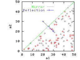
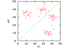
Consider the data shown in Figure 2(a) for two attributes
a1 and a2. The diamonds indicate the points actually
present in the data. This data is completely non-reflective: for any
point
![]() present in
the data, its reflection
present in
the data, its reflection
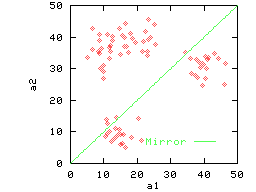
![]() does not exist. Figure 2(b) gives an
example of clustered data that is almost completely non-reflective.
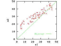
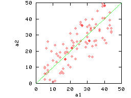
The correlated data in Figure 2(c) is also largely
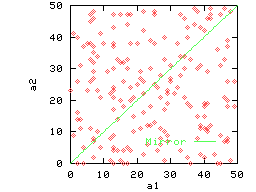
non-reflective. However, the data in Figure 2(d) is highly
reflective.
does not exist. Figure 2(b) gives an
example of clustered data that is almost completely non-reflective.
The correlated data in Figure 2(c) is also largely
non-reflective. However, the data in Figure 2(d) is highly
reflective.
| (a) Non-reflective | (b) Low Reflectivity |
 |
 |
| (c) Low Reflectivity | (d) High Reflectivity |
 |
 |
The implication of reflectivity is that the queries against a low
reflectivity data can be answered accurately without knowing the
attribute names, provided the realistic query conjecture is true.
Hence, although there is complete
overlap between the range of values of the two attributes in
Figures 2(a)-(c), we will get high accuracy on any
2-dimensional query. For example, consider the query
![]() on the data in Figure 2(a). This query can only
map to
on the data in Figure 2(a). This query can only
map to
![]() since there
are no points in the region around
since there
are no points in the region around
![]() .
.
Queries will often span a subset of the dimensions in the dataset, and
reflectivity will depend on the exact set of dimensions being
considered. Consider the query
![]() on the data in
Figure 2(a). This query can map to either
on the data in
Figure 2(a). This query can map to either
![]() or
or
![]() ,
and the answer
to this query will consist of points for which either a1 or
a2 is close to 20. Thus precision on this query will be around
50%, in contrast to the close to 100% precision that we can get on
the query
,
and the answer
to this query will consist of points for which either a1 or
a2 is close to 20. Thus precision on this query will be around
50%, in contrast to the close to 100% precision that we can get on
the query
![]() for the same dataset. Similar
behavior is exhibited by data in Figures 2(b)-(c): they are
highly non-reflective in 2 dimensions, but quite reflective in either of
the 1-dimensional projections.
for the same dataset. Similar
behavior is exhibited by data in Figures 2(b)-(c): they are
highly non-reflective in 2 dimensions, but quite reflective in either of
the 1-dimensional projections.
Before formally defining reflectivity, we make the following observations.
Let ![]() be a set of m-dimensional points of cardinality
be a set of m-dimensional points of cardinality
![]() .
Let
.
Let ![]() denote the co-ordinates of point xi.
We first define reflectivity over the full
m-dimensional space, and then give a
more general definition for subspaces.
denote the co-ordinates of point xi.
We first define reflectivity over the full
m-dimensional space, and then give a
more general definition for subspaces.
We define the reflections of the point xi to be the set of
co-ordinates obtained by permuting ![]() (including
(including ![]() ).
For example, if xi were
).
For example, if xi were
![]() ,
the reflections of xi would be {
,
the reflections of xi would be {
![]() ,
,
![]() }.
}.
Let
![]() denote the number of points within distance
r of
denote the number of points within distance
r of ![]() (in m-dimensional space).
The value of r is so chosen that the average value of
(in m-dimensional space).
The value of r is so chosen that the average value of
![]() (over all
(over all
![]() )
is close to the number of top answers that users will be interested in.
Let
)
is close to the number of top answers that users will be interested in.
Let
![]() denote the number of points
in
denote the number of points
in ![]() that have at
least one reflection within distance r of
that have at
least one reflection within distance r of ![]() .
The reflectivity of
.
The reflectivity of ![]() in m-dimensional space
is then defined to be:
in m-dimensional space
is then defined to be:
Now consider a k-dimensional subspace
S of the space of ![]() .
We define the
k-reflections of a point xi in
.
We define the
k-reflections of a point xi in ![]() to be the set of co-ordinates
obtained by considering the k! permutations of mCkcombinations of k co-ordinates chosen from
to be the set of co-ordinates
obtained by considering the k! permutations of mCkcombinations of k co-ordinates chosen from ![]() .
For example, the 2-reflections of a 3-dimensional point
.
For example, the 2-reflections of a 3-dimensional point
![]() will be the set
{
will be the set
{
![]() ,
,
![]() ,
,
![]() ,
,
![]() ,
,
![]() ,
,
![]() }.
}.
Let
![]() represent the co-ordinates of point xi projected
onto this subspace.
Let
represent the co-ordinates of point xi projected
onto this subspace.
Let
![]() denote the number of
points in
denote the number of
points in ![]() whose projections onto the subspace Sare within distance r of the co-ordinates
whose projections onto the subspace Sare within distance r of the co-ordinates
![]() (in the
k-dimensional space). As before, the value of r is so
chosen that the average value of
(in the
k-dimensional space). As before, the value of r is so
chosen that the average value of
![]() (over all
(over all
![]() )
is close to the number of desired top answers. that
Let
)
is close to the number of desired top answers. that
Let
![]() denote the number of points in
denote the number of points in ![]() that have at least one
k-reflection within distance rof the co-ordinates
that have at least one
k-reflection within distance rof the co-ordinates
![]() (in the k-dimensional space).
The reflectivity of the subspace S is defined to be:
(in the k-dimensional space).
The reflectivity of the subspace S is defined to be:
Finally, let
![]() represent the set of k-dimensional
subspaces of
represent the set of k-dimensional
subspaces of ![]() .
Let
.
Let
![]() denote
the number of k-dimensional subspaces
Then, the reflectivity of
denote
the number of k-dimensional subspaces
Then, the reflectivity of ![]() over k-dimensional subspaces
is defined to be the average of the reflectivity in each subspace:
over k-dimensional subspaces
is defined to be the average of the reflectivity in each subspace:
Note that:
Let S be the subspace corresponding to the attribute in a query
![]() .
Let
.
Let ![]() denote the co-ordinates corresponding to
denote the co-ordinates corresponding to
![]() .
Then there are
.
Then there are
![]() documents
that are true close matches to Q, and
documents
that are true close matches to Q, and
![]() documents that are nameless close matches to Q. Hence for this
query, the probability that a document that is a nameless close match
will also be a true close match is simply
documents that are nameless close matches to Q. Hence for this
query, the probability that a document that is a nameless close match
will also be a true close match is simply
![]() .
.
Let us represent a query distribution for a subspace S by a random
sample of queries
![]() drawn
from that distribution. Then for a query belonging to this
distribution, the probability that a document that is a nameless close
match will also be a true close match is
drawn
from that distribution. Then for a query belonging to this
distribution, the probability that a document that is a nameless close
match will also be a true close match is
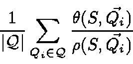
Finally, if the query distribution for a subspace S is close to the distribution of documents projected onto S, we can treat the set of points as a sample of the query distribution, and the probability that a document that is a nameless close match will also be a true close match is simply Non-reflectivity(S, r). Thus reflectivity can serve as a close proxy for expected accuracy.
If the database knows the correct attribute names corresponding to data values,
we can use Eq. 7 to compute reflectivity.
Null values in the data can be handled as follows.
Suppose the values of some of the co-ordinates of
an m-dimensional point xi are null (unknown).
We ignore this point in the computation of
reflectivity in Eq. 5.
When computing the reflectivity of a subspace S in
Eq. 6, the term
![]() for point xi
is excluded from the summation if a null value is present in the set of co-ordinates
projected onto S.
However, xi may still contribute to the denominator of the above term
for some other point xj if a k-reflection of xi does not have
any null co-ordinate values and this reflection is within distance
r of
for point xi
is excluded from the summation if a null value is present in the set of co-ordinates
projected onto S.
However, xi may still contribute to the denominator of the above term
for some other point xj if a k-reflection of xi does not have
any null co-ordinate values and this reflection is within distance
r of
![]() .
.
The cost of computing reflectivity can be reduced by doing the summation in Eq. 6 for a sample of data points. Similarly, we can do summation over a sample of subspaces in Eq. 7.
Consider now the scenario where attribute names have not been assigned to most of the values in the documents. If we can get hints for the attribute name, we can treat the highest-ranked hint for each number as the attribute name and compute reflectivity. We empirically evaluate this idea in Section 6.6. Our results show that this idea tends to be useful if the accuracy of hints is relatively high.
Finally, consider the situation in which we do not even have good hints. The proposed techniques may still work well; we just will not be able to estimate accuracy a priori. If the answers displayed to the user show sufficient summary information that the user's selections are a reliable indicator of the accuracy of the answer, we can use the precision of the answers as a rough estimate of reflectivity.
| (a) Clustered & Reflective | (b) Correlated & Reflective |
 |
 |
We now give algorithms for finding documents in response to a user query. These algorithms assume that the database as well as queries have no attribute names associated with the numbers. Section 5 discusses how to take advantage of this extra information.
Recall that a document D consists of
![]() (Eq. 2).
A search query Q consists of
(Eq. 2).
A search query Q consists of
![]() (Eq. 4).
Note that both D and Q are multi-sets.
Each value corresponds to an unspecified
attribute name.
(Eq. 4).
Note that both D and Q are multi-sets.
Each value corresponds to an unspecified
attribute name.
In computing the distance of query Q from a document D,
each q value is matched with exactly one n value.
Given a set of query numbers
![]() and a set of
matching document numbers
and a set of
matching document numbers
![]() ,
the distance function F with the Lp norm (
,
the distance function F with the Lp norm (
![]() )
is defined as
)
is defined as
Maximizing similarity is equivalent to minimizing distance.
Given a set
![]() of k numbers,
and a set
of k numbers,
and a set
![]() of m document numbers,
we want to select the numbers in D that will lead to the minimum distance.
Each number in D is allowed to match with a single number in
Q, and vice versa.
of m document numbers,
we want to select the numbers in D that will lead to the minimum distance.
Each number in D is allowed to match with a single number in
Q, and vice versa.
Construct a weighted bipartite graph G as follows:
Figure 4 shows the weighted bipartite graph for
Q={20,60} and D={10,25,75},
assuming the distance function
to be L1 and
![]() .
.
Lemma
The optimum solution to the minimum weight bipartite graph matching problem for
the graph G matches each number in Q with a
distinct number in D such that we get the lowest value for the
distance score F(Q,D).
We have marked in bold the edges comprising the optimum solution for the graph in Figure 4. Thus, 20 in Q is matched with 25 in D and 60 with 75 for a total distance score of 0.5.
We can now refer to the rich weighted bipartite graph matching literature (see survey in [4]) to find the best matching between the numbers in a query and the numbers in a document. We also obtain the distance score at the same time, which is used for ranking the documents. By repeating this process for every document in the database, we have a solution to our problem. In Section 4.2, we present techniques that avoid examining every document.
The best known algorithm for the weighted bipartite matching problem
is due to Feder and Motwani [13]
and its time complexity is
![]() ,
where e is the number of edges in the graph.
Since
,
where e is the number of edges in the graph.
Since
![]() ,
the complexity is
,
the complexity is
![]() .
.
We now address the question of how to limit the number of documents for which we have to compute the distance. This problem turns out to be similar to that of retrieving the top t objects that have highest combined score on k attributes, introduced in [11]. We first describe the score aggregation problem and the threshold algorithm for solving this problem [12] [14] [20].
Score Aggregation Problem
Assume that each object in a database has k scores, one for
each of k attributes.
For each attribute, there is a sorted list, which lists each object
and its score for that attribute, sorted by score (highest score first).
There is some monotone aggregation function f for combining
the individual scores to obtain an overall score for an object.
The problem is to efficiently find the top t objects that have the
best overall score.
Threshold Algorithm (TA)
There are two modes of access to data.
Sorted access obtains the score of an object in one of the sorted
lists by proceeding through the list sequentially from the top.
Random access obtains the score of an object in a list in one access.
The threshold algorithm works as follows
[12].
Proposed Adaptation
We now discuss how our problem is similar to the score aggregation problem.
We then show how the threshold algorithm can be adapted to our problem.
Assume that the documents have been processed to create data structures
to support the following types of accesses.
Here is the algorithm, stated in the TA framework. While reading the algorithm, keep in mind that a document with a lower distance score is closer to the query, and hence better in our setting.
At this point, for any document that has not been seen in the index, the
closest number to each query term qi must be at least as far from
qi as ni', and hence the distance between the document and
the query must be at least as high as ![]() .
.
Note that unlike the original threshold algorithm, the si scores in
the adaptation are lower bounds on the distance, not necessarily the
actual distance. In other words, when we match a document D to a
query, the number that ends up being matched with qi may be further
away from qi than indicated by the score for D in the sorted list
for qi. The reason is that during matching, a number in D can
only match
one query term, but we do not track this constraint during index access
(to avoid the bookkeeping overhead). Thus if a single number in D is
the closest number to two different query terms, one of the two scores
for D will be a lower bound for the actual distance. This
does not affect the correctness of the halting criteria in step 3, since
the threshold value ![]() is a lower bound on the distance of a
document that we have not yet seen, and we stop when we have seen
t documents whose distance is lower than
is a lower bound on the distance of a
document that we have not yet seen, and we stop when we have seen
t documents whose distance is lower than ![]() .
.
We now describe how to use hints about attribute names to aid matching.
Let Hi denote the set of attribute names associated with the
number ni in a document. As before, let Ai denote the set of
attribute names associated with qi in a query. We extend the
distance function from Eq. 9 to incorporate
hints as follows:
The parameter Bbalances the importance between the match on the numbers and the match on the hints. In general, the higher the accuracy of the hints and the higher the reflectivity of the data, the higher should be the value of B.
Recall that the function
w(qi,nj) determines the distance
between a query number and a document number.
Analogously,
v(Ai, Hj) is a function that determines the
distance between the set of attribute names associated with a query
number and the set of attribute names associated with a document number.
We use the following distance function v in our experiments:
 |
(11) |
Our techniques are independent of the specific form of the function v. A more sophisticated function form tuned to the specific data extractor being used (e.g., by incorporating belief values generated by the data extractor) may yield better results. However, as we will see, our experiments indicate that even this simple function can be quite effective.
Determining the weight B A good value for
B is important for successfully using hints. Suppose the
website provides enough summary with each answer that the user is
likely to click on relevant answers. By tracking
user clicks, we can get a set of queries for which we know the true
answers with high probability. Treat this set as a tune set and
evaluate the performance of the matching algorithm for different values
of B. Then pick the value that gives the highest accuracy.
If a set of values give similar accuracy, pick the median value in the set.
Note that the best value of B is likely to be different for
different query sizes, and hence we will need a tune set per query size.
Constructing the Bipartite Graph
As before, we map the matching problem to weighted bipartite graph
matching. The only difference is that we now assign
![]() as the weight of the edge
(qi,nj).
as the weight of the edge
(qi,nj).
Limiting the Set of Matches
The algorithm proposed in Section 4.2 can be used as is
even in the presence of hints, since we only need the sij score to
be a lower bound on the true distance. That is, we can use
sij =
w(qi, nij) to create the sorted list Li for qi,
ignoring the match on attribute names.
However, the algorithm will be considerably more efficient if we modify
it as follows. First, create an index to support an
additional type of access, hint
index access: given a number ni together with an attribute name
ai, return the set of documents in which ni is present and the set
of hints for ni includes ai.
The original index can be
(conceptually)
treated as a special case of this index, where the attribute
name
![]() .
.
Now, in Step 1, for each query term qi,
create an ordered list
![]() and associate the score
and associate the score
![]() with the entry
with the entry
![]() ,
such that
,
such that
![]() .
We can do this efficiently by using hint index access for
each attribute name in the set of hints Ai associated with the
query term qi, and also for the empty attribute name
.
We can do this efficiently by using hint index access for
each attribute name in the set of hints Ai associated with the
query term qi, and also for the empty attribute name ![]() .
Step 2 does not change. In Step 3, the only change is that we now
define the threshold value
.
Step 2 does not change. In Step 3, the only change is that we now
define the threshold value ![]() to be
to be
![]() from Eq 10, where
from Eq 10, where
![]() is
the entry in the index that we last looked at for query term qi.
is
the entry in the index that we last looked at for query term qi.
If the unit names are available in addition to attribute names,
we extend the distance function from Eq. 10 by adding
a term
![]() for whether the
units match:
for whether the
units match:
 |
(12) |
An additional complication arises due to different units (e.g., MHz and GHz) being assigned to the values of the same attribute. In some cases, this problem can be approached by converting the corresponding quantities into a `standard' form.
In this section, we report the results of experiments we performed to study the accuracy and performance characteristics of the proposed techniques. We used synthetic as well as real datasets in this study. Synthetic datasets are amenable to controlled experiments, while real datasets are good as a sanity check.
Given a database ![]() in which the correct correspondences between
the numbers and the attribute names are known,
a query Q consisting
of numbers and full information about the attribute names corresponding
to those numbers,
we could generate the ``perfect'' answer of top t matching documents
in which the correct correspondences between
the numbers and the attribute names are known,
a query Q consisting
of numbers and full information about the attribute names corresponding
to those numbers,
we could generate the ``perfect'' answer of top t matching documents
![]()
![]() for a given distance function F.
If the information about the attribute name is not available or only partially
available in the form of hints,
we would generate a different set of top tmatching documents
for a given distance function F.
If the information about the attribute name is not available or only partially
available in the form of hints,
we would generate a different set of top tmatching documents
![]() .
.
Precision(t) is defined to be the the percentage of documents in
MP(t) that are also present in M(t):
A document is modeled as a set of m numbers, corresponding to mknown attributes.
We generated three types of synthetic data:
Figure 5 shows the pseudocode for generating the
three types of synthetic data.
We use ![]() to control the amount of
reflectivity. The value of s[j] is initially set to
to control the amount of
reflectivity. The value of s[j] is initially set to
![]() ,
where R is a parameter that controls to the amount of overlap between
the range of values of various attributes, which in turn influences
reflectivity. If we wanted to generate a dataset with almost no overlap
between any of the attributes, R would be set to a high value, e.g.,
10. On the other hand, if we wanted very high overlap between the
attributes, R would be set to 0.
In our experiments, we manually tuned R such
that the 1-dimensional non-reflectivity is roughly 80% for each of the
three datasets (with the default number of attributes).
The values in
,
where R is a parameter that controls to the amount of overlap between
the range of values of various attributes, which in turn influences
reflectivity. If we wanted to generate a dataset with almost no overlap
between any of the attributes, R would be set to a high value, e.g.,
10. On the other hand, if we wanted very high overlap between the
attributes, R would be set to 0.
In our experiments, we manually tuned R such
that the 1-dimensional non-reflectivity is roughly 80% for each of the
three datasets (with the default number of attributes).
The values in
![]() are then randomly permuted, so that for the correlated dataset
there is no connection between which attributes are correlated and which
attributes are adjacent in terms of values.
are then randomly permuted, so that for the correlated dataset
there is no connection between which attributes are correlated and which
attributes are adjacent in terms of values.
// N: number of documents // m: number of attributes // Di: |
Figure 6 shows the settings used in the synthetic data experiments. The Range column gives the range of values used in various experiments. The Default column provides the default value of the corresponding parameter. Query size refers to the number of terms in the query.
To generate a query of size k, we first pick a document at random. Next, for Independent and Clustered, we randomly pick kattributes from the document, and for Correlated, we randomly pick a set of k consecutive attributes. We then remove this document from the dataset, and compute the precision. (If we kept the document in the dataset, our scores would be artificially boosted.) We average the results over 1000 queries for each combination of parameters and query size. We use L1 to compute distance between a query and a document in all our experiments.
Figure 7 gives information about the nine real datasets used in our experiments. The first four datasets came from the Pangea data on electronic components for different categories of electronic parts. The last five datasets are from the University of California-Irvine Repository of Machine Learning. A record here corresponds to a document.
The query generation procedure used with the real data is identical to the procedure we described for the Independent and Clustered data. All results are the average of 1000 queries.
Figure 8(a) shows the precision on the three synthetic datasets as the query size is increased. We compute answers to the same query under two settings: (i) attribute names are known for both data and query, and (ii) attribute names are ignored in data as well as query. We then use Eq. 13 to compute precision. Figure 8(b) plots non-reflectivity versus subspace dimensionality. Non-reflectivity is computed assuming attribute names are known in the data. Both precision and non-reflectivity have been plotted as a percentage. These figures show that precision at a given query size closely tracks non-reflectivity for the corresponding subspace dimensionality.
As anticipated, both Clustered and Correlated gave higher precision than Independent. Clustered gave higher precision than Correlated for higher query dimensions. To understand the behavior of Clustered with increasing subspace dimensionality, recall our example from Figure 2(b). This dataset has very low reflectivity in 2 dimensions, but high reflectivity in one dimension. Similarly, in our synthetic data, the clusters gradually merge as we drop dimensions, leading to an increase in reflectivity for lower dimensions. By the time we reach 2 dimensions, the clusters have completely disappeared and Clustered starts behaving like Correlated and Independent.
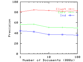
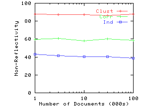
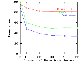
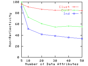
Figure 9(a) shows the precision as a function of the number of documents. Figure 10(a) shows the precision as a function of the number of data attributes. We again note from corresponding figures that the precision closely tracks non-reflectivity.
| (a) Precision | (b) Reflectivity |
 |
 |
| (a) Precision | (b) Reflectivity |
 |
 |
We now study the effectiveness of indexing in limiting the set of documents for which we have to compute the distance for a query. All our experiments were run on a 933 MHz Pentium III with 512 MB of memory. The code was written in Java and run with Sun JDK 1.3 Hotspot Server. The execution times will be faster with C++, but the relative impact of various factors is likely to be the same. Both index and documents were kept completely in memory, limiting us to around 800,000 documents.
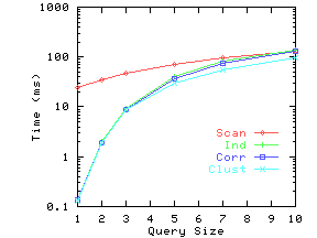
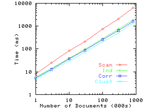
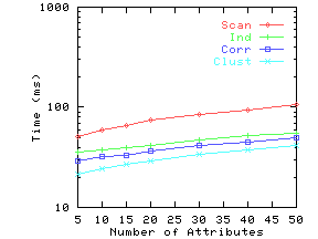
Figure 11 shows the execution times with and without indexing for the Independent, Correlated and Clustered datasets. The time without indexing was almost identical for the three datasets, and hence we only plot one curve, ``Scan'' for the no indexing case.
| (a) Varying query size (#documents = 10K, #attributes = 20) | (b) Varying number of documents (Query Size = 5, #attributes = 20) |
 |
 |
| (c) Varying number of attributes (Query Size = 5, #documents = 10K) | |
 |
|
Figure 11(a) shows the execution time results for different query sizes for the three synthetic datasets. The index is quite effective for smaller query sizes, which we expect to be the norm. For larger query sizes, the dimensionality curse begins to catch up and using the index only does a little better than a full scan.
Figure 11(b) shows the scalability of the indexing as we increase the number of documents from 1000 to almost 1 million. At query size 5, the number of documents matched goes up by a factor of about 250 times as we increase the number of documents by 800 times, and the number of index entries scanned goes up around 200 times. Hence while the fraction of the index scanned and the percentage of documents checked both decrease slightly, the absolute time goes up almost linearly with the number of documents. At 800,000 documents, we take slightly more than 1 second for query size 5 and around 0.03 seconds for query size 2.
Figure 11(c) shows that the execution time remains flat as we increase the number of attributes. In our synthetic datasets, adding new attributes does not change the average amount of overlap between attributes. Hence the number of documents matched or index entries scanned is not affected by adding more attributes. However, matching takes a little longer, and hence the overall time goes up slightly.
Figure 12 shows results on three of the real datasets. For DRAM, there were often a large number of documents at a distance of zero from the query Q for smaller query sizes. Hence whether we stop as soon as we get 10 documents with zero distance, or whether we get all documents at zero distance (and then present a random sample), makes a dramatic difference in the running time. The ``All Closest'' line shows the former case, and the ``Any 10'' line the latter. For the other two datasets, this is not a significant issue, and hence these two lines are very close to each other. Again, we can conclude that indexing is quite effective for smaller query sizes.
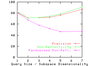
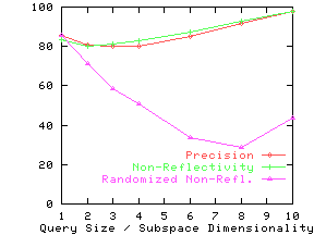
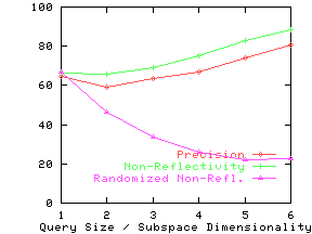
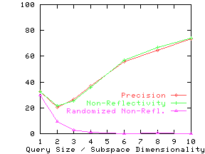
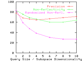
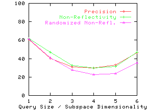
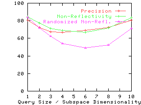
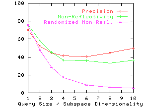
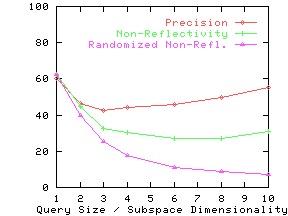
Figure 13 shows the precision and non-reflectivity as a percentage in the same graph for the nine real datasets. The x-axis for precision and non-reflectivity is query size and subspace dimensionality respectively. We again see that non-reflectivity can provide a good estimate of the expected precision. We also see that real datasets can be quite non-reflective and hence our techniques can be effectively used on them.
| (a) DRAM | (b) LCD |
 |
 |
| (c) Microprocessor | (d) Transistor |
 |
 |
| (e) Automobile | (f) Credit |
 |
 |
| (g) Glass | (h) Housing |
 |
 |
| (i) Wine | |
 |
|
Effect of Clustering and Correlation
In Section 3, we stated our intuition that clustering
and correlation would typically increase non-reflectivity. To verify
this conjecture, we study
the effect of destroying any clustering or correlation effects in a
dataset by randomly permuting the values for every attribute.
(We permute the values of an attribute across documents, not across
different attributes.)
If the attributes were originally independent, this permutation will not affect
reflectivity, since permutation does not affect the distribution of
values for
each attribute. Hence the difference in non-reflectivity between the
original data and the randomized data can be attributed to clustering
and correlation. The line ``Randomized Non-Refl.'' shows the
non-reflectivity on the randomized datasets. For all but the Credit
dataset, randomized non-reflectivity is substantially lower than
non-reflectivity.
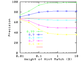
We generated data for this set of experiments by starting with the real datasets and then augmenting them with hints. Our procedure for generating hints takes two parameters: AvgNumHints and ProbTrue. AvgNumHints is the average number of hints per data value. Each data value is assigned at least one hint, hence the minimum value of AvgNumHints is 1. If AvgNumHints is greater than 1, then the number of hints for a specific data value is determined using a Poisson distribution. ProbTrue is the probability that the set of hints for a data value includes the true attribute name. Figure 14 gives the pseudocode for generating hints for a given data value. In general, increasing AvgNumHints should result in increasing ProbTrue. However, since the exact relationship is data and data extractor dependent, in any given experiment, we fix one of the values and vary the other. The query consists of numbers together with the corresponding true attribute name.
// ProbTrue: Prob. of true attribute name being in the set of hints |
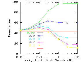
We synthesized nine datasets from the real datasets described earlier, and experimented with all of them. However, we show the graphs for only three representative datasets: DRAM, Auto and Wine. DRAM and Auto have high non-reflectivity, and Wine lower non-reflectivity.
Weighting the Match on Hints
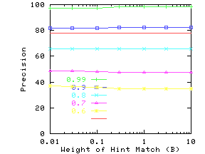
Figure 15 shows the effect of changing the
weight given to the match on the attribute names (the parameter
B in Eq. 10). AvgNumHints was set to 1, so
that every data value had exactly one hint assigned to it.
The different curves show precision for different values of ProbTrue.
If the hints are accurate (high value of ProbTrue), then precision
rapidly goes up with increasing B. For DRAM, the precision goes up
for values of B much smaller than 0.01, and hence
Figure 15(a) does not show this increase.
For queries on DRAM, there are often different attributes with the same
numeric value as the query value, and
even a small value of B is sufficient to pick between them.
If the hints are not very accurate, precision goes down with
increasing B. One should not conclude that B should be
![]() if hints are accurate and 0 otherwise. For example,
in the case of wine with ProbTrue between 0.6 and 0.8, the
precision initially goes up with B and then drops back down.
Therefore it is important to choose a good value of B.
if hints are accurate and 0 otherwise. For example,
in the case of wine with ProbTrue between 0.6 and 0.8, the
precision initially goes up with B and then drops back down.
Therefore it is important to choose a good value of B.
In the rest of the experiments, we assume we have a tune set of 100 queries (per query size) for which we know the best match. We compute Precision over this tune set for different values of B(specifically, we used { 0.01, 0.03, 0.1, 0.3, 1, 3, 10 }). We then choose the value that gives the highest precision. As we mentioned in Section 5, this method can be used as long as the website provides enough summary with each answer so that the user is likely to click on relevant answers.
| (a) DRAM (query size 2) | (b) Auto (query size 2) |
 |
 |
| (c) Wine (query size 5) | |
 |
|
Effectiveness of Hints
Figure 16 shows the gains in precision
for different values of ProbTrue when AvgNumHints is set to 1.
Notice that for datasets with high non-reflectivity (DRAM and Auto), the hints
have to be extremely accurate (ProbTrue > 0.9) to add significant value.
However, for datasets with low non-reflectivity (Wine), even hints with
lower levels of accuracy can increase precision.
Number of Hints
In the previous set of experiments, we found that ProbTrue (the
probability that the set of hints will include the true attribute name)
had to be
quite high to increase precision. In many domains, such high values of
ProbTrue may not be achievable without
having multiple hints per attribute, where only one of the hints is correct.
Figure 17 shows precision for different values of
the average number of hints (AvgNumHints). For each line, we have fixed
the value of ProbTrue.
As expected, for a fixed value of ProbTrue,
precision decreases as the number of hints increases. However, we
expect ProbTrue to increase with the number of hints.
Consider Figure 17(c), and assume we have a data extractor
that gives ProbTrue of 0.7 when AvgNumHints = 1, ProbTrue of 0.9 when
AvgNumHints = 1.5, and ProbTrue of 0.99 when AvgNumHints ![]() 3. In this
scenario, choosing AvgNumHints = 3 will result in the highest
precision.
Thus, having multiple hints can improve precision if there is an
accompanying increase in ProbTrue.
3. In this
scenario, choosing AvgNumHints = 3 will result in the highest
precision.
Thus, having multiple hints can improve precision if there is an
accompanying increase in ProbTrue.
Estimating Reflectivity using Hints
Finally, we explore how well we can estimate non-reflectivity
when we do not know true attributes but only have
hints about them. We generate data with AvgNumHints = 1 and different
values of
ProbTrue, treat each hint as if it were the true attribute name, and
compute reflectivity. Figure 18 shows the results.
The values on the y-axis, with ProbTrue = 1, are the true values of
non-reflectivity. The non-reflectivity estimates are
lower with hints than with true attribute names. However, for small
subspace dimensions, the drop-off is sufficiently gradual that the
estimate is still useful when the hints are reasonably accurate. For
larger subspace dimensions, the drop-off is sometimes quite steep. Hence
if the estimate for non-reflectivity has a low value, we cannot be sure
that the true value of non-reflectivity is indeed low or whether it is
an artifact of the inaccuracy of hints.
But if we get a high value, we
can be confident that the true value of non-reflectivity is also high.
We identified a data property, called reflectivity, that can tell a priori how well our approach will work against a dataset. High non-reflectivity in data assures that our techniques will have high precision. Our experiments showed that real datasets can exhibit high non-reflectivity and our techniques yielded high precision against these datasets. Using synthetic data, we also showed the scalability and resilience of our techniques in terms of the number of documents, number of attributes in the data, size of queries, and types of data.
We also showed how we can use imprecise attribute names as hints to improve precision. Hints are particularly helpful when the data has low non-reflectivity. However, for datasets with high non-reflectivity, hints have to be extremely accurate to improve precision beyond what we get by matching numbers.
In the future, we plan to extend this work in three directions. First, we would like to handle queries in which value ranges are provided. Second, some extraction procedures associate confidence values with the attribute names assigned to a number. We wish to explore how to take advantage of this additional information. Finally, we would like to better understand the interaction between correlated and clustered data and reflectivity.
Acknowledgment We wish to thank Ron Fagin for discussions on the threshold algorithm.